21.3.1 Using the Soot Models

When the mass fraction of soot is relatively large (e.g., 10%) or if your problem involves the effect of radiation, the soot formation should be computed as part of the main combustion solution and not through postprocessing (as is done for the NOx and SOx models). The procedure for setting up and solving a soot formation model is outlined below, and described in detail on the pages that follow. Remember that only the steps that are pertinent to soot modeling are shown here. For information about inputs related to other models that you are using in conjunction with the soot formation model, see the appropriate sections for those models.

1.   Set up your combustion problem using ANSYS FLUENT as usual. Note the following limitations:

• None of the soot models are compatible with premixed combustion.

• Only the Moss-Brookes model and the Hall extension are compatible with non-premixed and partially premixed combustion.

• The one-step and two-step soot formation models are only available for turbulent flows.

2.   Enable the desired soot formation model and set the related parameters, as described in this section.

Models Soot Edit...

3.   Define the boundary conditions for soot (and nuclei, if you are not using the one-step model) at flow inlets.

Boundary Conditions

4.   In the Solution Controls task page, set a suitable value for the soot (and nuclei, if you are not using the one-step model) under-relaxation factor(s). The default value is 0.9, although a lower value may be required for certain problems. That is, if convergence cannot be obtained, try a lower under-relaxation value.

Solution Controls

5.   Perform calculations until convergence (i.e., until the soot / nuclei residual is below $10^{-6}$) to ensure that the soot (and nuclei) field is no longer evolving.

Run Calculation

6.   Review the mass fraction of soot (and nuclei) with alphanumerics and/or graphics tools in the usual way.

7.   Save a new set of case and data files, if desired.

Setting Up the One-Step Model

You can enable and set up the one-step soot formation model by using the Soot Model dialog box (Figure  21.3.1).

Models Soot Edit...

Figure 21.3.1: The Soot Model Dialog Box for the One-Step Model

Under Model, select One-Step. The dialog box will expand to show the appropriate inputs.

Next, you need to tell ANSYS FLUENT which chemical species in your model should be used as the fuel and oxidizer. Under Species Definition, select the fuel in the Fuel drop-down list and the oxidizer in the Oxidant drop-down list. If you are using the non-premixed model for the combustion calculation and your fuel stream consists of a mixture of components, you should choose the most appropriate species as the Fuel species for the soot formation model. Similarly, the most significant oxidizing component (e.g., O $_2$) should be selected as the Oxidant.

If you want to include the effects of soot formation on the radiation absorption coefficient, enable Soot-Radiation Interaction in the Options group box. For more details, see this section in the separate Theory Guide.

You must next define the Process Parameters, input the stoichiometry of the fuel and soot combustion for the one-step model:

Stoichiometry for Soot Combustion   is the mass stoichiometry, $\nu_{\rm soot}$, in this equation in the separate Theory Guide , which computes the soot combustion rate. The default value supplied by ANSYS FLUENT (2.6667) assumes that the soot is pure carbon and that the oxidizer is O $_2$.

Stoichiometry for Fuel Combustion   is the mass stoichiometry, $\nu_{\rm fuel}$, in this equation in the separate Theory Guide , which computes the soot combustion rate. The default value supplied by ANSYS FLUENT (3.6363) is for combustion of propane (C $_3$H $_8$) by oxygen (O $_2$).

You must then set the Modeling Parameters that are used in this equation , this equation , and this equation in the separate Theory Guide :

Soot Formation Constant   is the parameter $C_s$ in this equation in the separate Theory Guide.

Equivalence Ratio Exponent   is the exponent $r$ in this equation in the separate Theory Guide.

Equivalence Ratio Minimum   and Equivalence Ratio Maximum are the minimum and maximum values of the fuel equivalence ratio $\phi$ in this equation in the separate Theory Guide. This equation will be solved only if Equivalence Ratio Minimum $< \phi <$ Equivalence Ratio Maximum; if $\phi$ is outside of this range, there is no soot formation.

Activation Temperature of Soot Formation Rate   is the term $E/R$ in this equation in the separate Theory Guide.

Magnussen Constant for Soot Combustion   is the constant $A$ used in the rate expressions governing the soot combustion rate ( this equation and this equation in the separate Theory Guide).

Note that the default values for these parameters are for propane fuel [ 15, 90], and are considered to be valid for a wide range of hydrocarbon fuels.

Setting Up the Two-Step Model

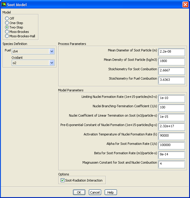
You can enable and set up the two-step soot formation model by using the Soot Model dialog box (Figure  21.3.2).

Models Soot Edit...

Figure 21.3.2: The Soot Model Dialog Box for the Two-Step Model

Under Model, select Two-Step. The dialog box will expand to show the appropriate inputs.

Note that the two-step Tesner model should only be used when the eddy-dissipation model is used to define the turbulence-chemistry interaction.

Next, you need to tell ANSYS FLUENT which chemical species in your model should be used as the fuel and oxidizer. Under Species Definition, select the fuel in the Fuel drop-down list and the oxidizer in the Oxidant drop-down list. If you are using the non-premixed model for the combustion calculation and your fuel stream consists of a mixture of components, you should choose the most appropriate species as the Fuel species for the soot formation model. Similarly, the most significant oxidizing component (e.g., O $_2$) should be selected as the Oxidant.

If you want to include the effects of soot formation on the radiation absorption coefficient, enable Soot-Radiation Interaction in the Options group box. For more details, see this section in the separate Theory Guide.

You must next define the Process Parameters, input the stoichiometry of the fuel and soot combustion, as well as the average size and density of the soot particles, for the two-step model:

Mean Diameter of Soot Particle   and Mean Density of Soot Particle are the assumed average diameter and average density of the soot particles in the combustion system, used to compute the soot particle mass, $m_p$, in this equation in the separate Theory Guide for the two-step model. Note that the default values for soot density and diameter are taken from [ 47].

Stoichiometry for Soot Combustion   is the mass stoichiometry, $\nu_{\rm soot}$, in this equation in the separate Theory Guide , which computes the soot combustion rate. The default value supplied by ANSYS FLUENT (2.6667) assumes that the soot is pure carbon and that the oxidizer is O $_2$.

Stoichiometry for Fuel Combustion   is the mass stoichiometry, $\nu_{\rm fuel}$, in this equation in the separate Theory Guide , which computes the soot combustion rate. The default value supplied by ANSYS FLUENT (3.6363) is for combustion of propane (C $_3$H $_8$) by oxygen (O $_2$).

You must then set the Modeling Parameters that are used in this equation , this equation , this equation , this equation , and this equation in the separate Theory Guide :

Limiting Nuclei Formation Rate   is the limiting value of the kinetic nuclei formation rate $\eta_0$ in this equation in the separate Theory Guide. Below this limiting value, the branching and termination term, ( $f-g$) in this equation in the separate Theory Guide , is not included.

Nuclei Branching-Termination Coefficient   is the term $(f - g)$ in this equation in the separate Theory Guide.

Nuclei Coefficient of Linear Termination on Soot   is the term $g_0$ in this equation in the separate Theory Guide.

Pre-Exponential Constant of Nuclei Formation   is the pre-exponential term $a_0$ in the kinetic nuclei formation term, this equation in the separate Theory Guide.

Activation Temperature of Nuclei Formation Rate   is the term $E/R$ in the kinetic nuclei formation term, this equation in the separate Theory Guide.

Alpha for Soot Formation Rate   is $\alpha$, the constant in the soot formation rate equation, this equation in the separate Theory Guide.

Beta for Soot Formation Rate   is $\beta$, the constant in the soot formation rate equation, this equation in the separate Theory Guide.

Magnussen Constant for Soot and Nuclei Combustion   is the constant $A$ used in the rate expressions governing the soot combustion rate ( this equation and this equation in the separate Theory Guide).

The default values for the two-step model are the same as in Magnussen and Hjertager [ 47] (for an acetylene flame), except for $a_0$, which is assumed to have the original value from Tesner et al. [ 87]. If your model involves propane fuel rather that acetylene, it is recommended that you change the value of $\alpha$ to $3.5 \times 10^8$ [ 5]. For best results, you should modify both of these parameters, using empirically determined inputs for your specific combustion system.

Setting Up the Moss-Brookes Model and the Hall Extension

You can enable and set up the Moss-Brookes and Moss-Brookes-Hall soot formation models by using the Soot Model dialog box (Figure  21.3.3).

Models Soot Edit...

Figure 21.3.3: The Soot Model Dialog Box for the Moss-Brookes Model

Under Model, select Moss-Brookes or Moss-Brookes-Hall. The dialog box will expand to show the appropriate inputs. Note the following about these models:

• The Moss-Brookes model was originally proposed for soot prediction in methane flames. However, it can be equally applicable to higher hydrocarbon species by appropriately modifying the soot precursor and participating surface growth species.

• The Moss-Brookes-Hall model is applicable for higher hydrocarbon fuels (e.g., kerosene) and will only be available when C $_2$H $_2$, C $_6$H $_6$, C $_6$H $_5$, and H $_2$ are present in the gas phase species list.

You must next define the precursor species in the Species Definition group box. When suitable precursor species are present in the species list, you can select species-list from the Precursor from drop-down list, and then select the Soot Precursor species and the Surface Growth species from the selection lists. Note that for the Moss-Brookes model, you can select acetylene ( c2h2), ethylene ( c2h4), and/or benzene ( c6h6) for the Soot Precursor; if neither are present or if you would specify a different precursor correlation, then curve fitting will be used to determine the precursor and surface growth species mass fractions (see Section  21.3.1 for further details regarding curve fitting).

Next, specify how turbulent fluctuations will be accounted for in the soot formation calculations, by defining the turbulence parameters in the Turbulence Interaction Mode group box.

Select one of the options in the PDF Mode drop-down list:

• Select none to ignore turbulence and use laminar soot rate calculations.

• Select temperature to take into account fluctuations of temperature.

• Select temperature/species to take into account fluctuations of temperature and mass fraction of the species selected in the Species drop-down list (which appears when you select this option).

• (non-premixed and partially premixed combustion calculations only) Select mixture fraction to take into account fluctuation in the mixture fraction(s). This is the recommended approach, as it generally yields the best results and accuracy.

When modeling the formation of other pollutants along with soot, you should compare the selections made in the PDF Mode drop-down lists in the Turbulence Interaction Mode tab of the NOx Model dialog box and the Turbulence Interaction Mode group boxes of the SOx Model and Soot Model dialog boxes. If mixture fraction is selected in any of these dialog boxes, then it must be selected in all of the others as well.

The mixture fraction option is available only if you are using either the non-premixed or partially premixed combustion model to model the reacting system. If you use the mixture fraction option, the instantaneous temperatures and species concentrations are taken from the PDF look-up table as a function of mixture fraction and enthalpy and the instantaneous soot production rates are calculated at each cell. The PDF used for convoluting the instantaneous soot rates is the same as the one used to compute the mean flow-field properties. For example, for single-mixture fraction models the beta PDF is used, and for two-mixture fraction models, the beta or the double delta PDF can be used. The PDF in terms of mixture fraction is calculated from the values of mean mixture fraction and variance at each cell, and the instantaneous soot rates are convoluted with the mixture fraction PDF to yield the mean rates in turbulent flow.

If you selected temperature or temperature/species for the PDF Mode, you should define the following parameters in the Turbulence Interaction Mode group box:

PDF Type   allows you to specify the shape of the PDF, which is then integrated to obtain mean rates for the temperature and (if you selected temperature/species for the PDF Mode) the species. If you select beta, the PDF will be modeled using this equation in the separate Theory Guide. If you select gaussian, the PDF will be modeled using this equation in the separate Theory Guide.

PDF Points   allows you to specify the number of points used to integrate the beta or Gaussian function in this equation or this equation in the separate Theory Guide on a histogram basis. The default value of 10 will yield an accurate solution with reasonable computation time. Increasing this value may improve accuracy, but will also increase the computation time.

Temperature Variance   allows you to specify the form of transport equation that is solved to calculate the temperature variance. The default selection is algebraic, which is an approximate form of the transport equation (see this equation in the separate Theory Guide). You have the option of selecting transported to instead solve this equation in the separate Theory Guide. Though the transported form is more exact, it is also more expensive computationally.

Tmax Option   provides various options for determining the maximum limit(s) for the integration of the PDF used to calculate the temperature. The default selection is global-tmax, which sets the limit as the maximum temperature in the flow field. You can select local-tmax if you would rather obtain cell-based maximum temperature limits by multiplying the local cell mean temperature by the value entered in Tmax Factor. You can select specified-tmax to set the limit for each cell to be the value entered in Tmax. Finally, if you have compiled a user-defined function for the soot rate and loaded the library into ANSYS FLUENT, then you can select user-defined so that the limit is specified by a UDF.

Species   only appears if you have selected temperature/species for the PDF Mode. Your selection in this drop-down menu determines which species' mass fraction is included in the soot formation calculations.

Note that the species variance will always be calculated using the algebraic form of the transport equation ( this equation in the separate Theory Guide).

Under Process Parameters, you must enter information about the mass and mean density of the soot particles:

Mass of Incipient Soot Particles   is $M_{\rm P}$ in this equation and this equation in the separate Theory Guide. Note that this value was assumed to be 144 kg/kgmol (12 carbon atoms) in the work of Brookes and Moss, whereas the Hall extension model assumed it to be 1200 kg/kgmol (100 carbon atoms).

Mean Density of Soot Particle   is $\rho_{\rm soot}$ in this equation in the separate Theory Guide and $\rho$ in this equation in the separate Theory Guide. Note that this value was assumed to be 1800 kg/m $^3$ in the work of Brookes and Moss [ 12], whereas Hall et al. [ 29] assumed it to be 2000 kg/m $^3$.

Next, you must select the Soot Oxidation Model. Your choices include the Fenimore-Jones model, as originally used in Brookes and Moss' work, or the Lee extended model. The Lee model will model soot oxidation due to hydroxyl radicals as in the Fenimore-Jones model, as well as the oxidation due to molecular oxygen.

You must then set the Modeling Parameters:

[OH] Model   allows you to specify the method by which the OH radical concentration is calculated. The recommended selection from the drop-down list is instantaneous, although this option is only available when OH is available in the species list and is calculated by the combustion model. The other option is the partial-equilibrium model, which necessitates the availability of [O] atom concentration within the field.

[O] Model   must be defined when you have selected partial-equilibrium for the [OH] Model, and specifies the method by which the O radical concentration is calculated. The options include equilibrium, partial-equilibrium, and instantaneous.

Note that in ANSYS FLUENT, the oxidation rate scaling parameter ( $C_{\rm oxid}$ in this equation in the separate Theory Guide) is set to unity. If you would like to change the value of this parameter, you can use the
define/models/soot-parameters/soot-model-parameters text command. A lower value will reduce the amount of soot oxidation.

If you want to include the effects of soot formation on the radiation absorption coefficient, enable Soot-Radiation Interaction in the Options group box. For more details, see this section in the separate Theory Guide.

Species Definition for the Moss-Brookes Model with a User-Defined Precursor Correlation

ANSYS FLUENT accepts the following as possible precursor species for the Moss-Brookes model: C $_2$H $_2$, C $_6$H $_6$, and C $_2$H $_4$. If none of these species are present in the species list (as is often the case when using the eddy-dissipation model) or if you would prefer to specify a different precursor correlation, your setup for the Moss-Brookes model will be different than noted previously. Under such circumstances, you should select user-correlation from the Precursor from drop-down list in the Species Definition group box (note that this is only option possible when the appropriate species are not present). The Soot Model dialog box will then be as shown in Figure  21.3.4.The parameters you set in the Species Definition group box allow ANSYS FLUENT to calculate a mixture fraction based on the mass fractions of the oxidant and the carbon/hydrogen contributed by a designated fuel species. The precursor species mass fraction will then be computed as a function (which you will also define) of this mixture fraction.

Figure 21.3.4: The Soot Model Dialog Box for the Moss-Brookes Model with a User-Defined Precursor Correlation

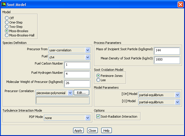In the Species Definition group box, you will first select a Fuel species and enter the related Fuel Carbon Number and Fuel Hydrogen Number for use in the mixture fraction calculation. Next, enter the Molecular Weight of Precursor (the default value is for acetylene). Then make a selection in the Precursor Correlation drop-down list to indicate how the precursor mass fraction will be related to the mixture fraction. A piecewise-polynomial profile is defined by default.

Note that the default values for the piecewise-polynomial profile are only valid for a methane diffusion flame simulation, in which both the air and fuel initial temperatures are set to 290 K, and acetylene is assumed as the soot precursor.

If you decide not to use the default values for Precursor Correlation, you must define the correlation between the precursor mass fraction and the mixture fraction. This correlation should be based on a laminar flamelet profile that you have generated, using either the equilibrium chemistry model in ANSYS FLUENT (see Section  16.2 for details) or another third-party software package of your choosing. You should then apply a curve-fitting technique to your generated profile, to obtain either a constant value or a piecewise-polynomial function.

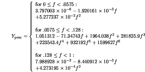
In a piecewise-polynomial function, the laminar flamelet profile is divided into a number of mixture fraction ranges. In each range, the precursor species mass fraction $Y_{\rm prec}$ is defined using the following equation:

where $NC$ is the number of coefficients $C$, and $f$ is the mixture fraction. The following piecewise-polynomial function corresponds to the default settings in ANSYS FLUENT:

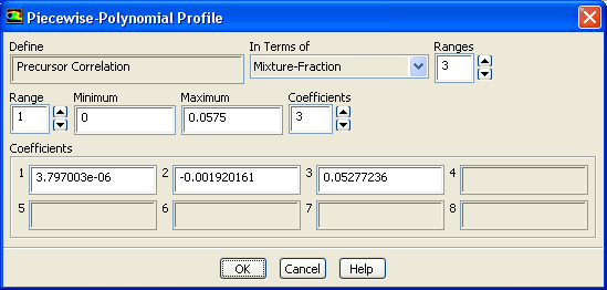
To define a piecewise-polynomial profile to relate the precursor mass fraction to the mixture fraction, select piecewise-polynomial from the Precursor Correlation drop-down list and click the Edit... button. The Piecewise-Polynomial Profile dialog box (Figure  21.3.5) will open.

Figure 21.3.5: The Piecewise-Polynomial Profile Dialog Box

Then perform the following steps in the Piecewise-Polynomial Profile dialog box:

1.   Enter the number of Ranges. For the example shown in Equation  21.3-2, three ranges of mixture fraction are defined, which is the maximum allowed.

2.   For the first range ( Range = 1), enter the Minimum and Maximum mixture fraction values, and the number of Coefficients. (Up to eight coefficients are available.) The number of coefficients defines the order of the polynomial. An input of 1 defines a polynomial of order 0, and the mass fraction will be constant and equal to the single coefficient. An input of 2 defines a polynomial of order 1, and the mass fraction will vary linearly with mixture fraction, and so on.

3.   Define the values for the coefficients in the Coefficients group box. The dialog box in Figure  21.3.5 shows the inputs for the first range of Equation  21.3-2.

4.   Increase the value of Range and enter the Minimum and Maximum mixture fractions, number of Coefficients, and the values for the Coefficients for the next range. Repeat if there is a third range.

Note when defining the ranges, you must start with the lowest mixture fraction range, and then proceed in order to the highest range. The solver will not sort them for you.

To define a constant profile to relate the precursor mass fraction to the mixture fraction, select constant from the Precursor Correlation drop-down list and enter a value in the accompanying text entry box.

Using the Coal-Derived Soot Extension of the Moss-Brookes Model (Beta Feature)

The steps that follow describe how to use the coal-derived soot extension of the Moss-Brookes model. For details about the theory and equations related to this extension, see this section in the separate Theory Guide.

1.   (optional) Set up and solve a combustion simulation that solves for the tar species.

2.   Enable and set up the discrete phase model, using the Discrete Phase Model dialog box. Make sure that the injections have coal or heavy oil specified as the injection material. See Chapter  23 for details.

3.   In the Soot Model dialog box, select Moss-Brookes in the Model list and set up the definitions and parameters. See Section  21.3.1 for details.

Note the following for the inputs in the Process Parameters group box:

• Enter 1080000 kg/kgmol for the Mass of Incipient Soot Particle, as this represents 9 $\times$ 10 $^{4}$ carbon atoms.

• A value of 1950 kg/m $^{3}$ is recommended for the Mean Density of Soot Particle.

4.   Enable the coal-derived soot extension using the following text command:

define $\rightarrow$ models $\rightarrow$ soot-parameters $\rightarrow$ soot-model-parameters

You can use the settings for most of the prompts that follow this text command, as they reflect the settings you made in the Soot Model dialog box and the default Moss-Brookes model settings. The prompts that relate to the coal-derived soot extension are the following:

(a)    Coal-derived soot?

Enter yes to enable the coal-derived soot extension.

(b)    Solve tar equation?

Enter yes if you need to solve for the tar species. Enter no if you have already run a combustion simulation that calculated the tar species. Your answer will affect the inputs to the define/models/soot-parameters/
soot-process-parameters text command (as described below).

(c)    Collision Constant

Enter a value for the collision constant. The recommended value is 3.

5.   Set the process parameters for the coal-derived soot extension using the following text command:

define $\rightarrow$ models $\rightarrow$ soot-parameters $\rightarrow$ soot-process-parameters

You can use the settings for some of the prompts that follow this text command, as they reflect the settings you made in the Soot Model dialog box. The prompts that relate to the coal-derived soot extension will vary, depending on whether you have already run a combustion simulation that calculated the tar species.

• If you requested that the tar equations be solved using the define/models/
  soot-parameters/soot-model-parameters text command, then the prompts that relate to the coal-derived soot extension are the following:

  (a)    Number of tar streams

  Enter the number of tar streams for the model. This value will depend on the number of different coal or heavy oil injections defined using the Injections dialog box.

  (b)    Mass fraction of tar in coal volatiles

  For each tar stream, enter the mass fraction of tar in the coal volatiles. It is recommended that this value be between 0.3 and 0.5.

  (c)    Species name

  For each tar stream, enter the name of the fuel species of the associated volatile stream. The tar evolution will then be calculated as a fraction of the volatiles that evolve from this fuel species.

  (d)    Remove fuel species from list?

  If you made a mistake when entering the number of tar streams or the species name, you can remove the erroneous species from the calculation by entering yes.

• If you requested that the tar equations not be solved using the define/models/
  soot-parameters/soot-model-parameters text command, then the prompt that relates to the coal-derived soot extension is the following:

  Tar species name

  Enter the name of the tar species from your previous combustion model solution.

6.   Specify the desired turbulent Schmidt number for the soot mass fraction and nuclei transport, using the following text command:

define $\rightarrow$ models $\rightarrow$ soot-parameters $\rightarrow$ modify-schmidt-number?

The suggested value is 700.

Defining Boundary Conditions for the Soot Model

At flow inlet boundaries, you will need to specify the Soot Mass Fraction and (when not using the one-step model) the Nuclei mass concentration. These correspond to $Y_{\rm soot}$ in this equation and this equation in the separate Theory Guide and $b_{\rm nuc}^*$ in this equation and this equation in the separate Theory Guide , respectively.

Boundary Conditions

You can retain the default inlet values of zero for both quantities or you can input nonzero numbers as appropriate for your combustion system.

Reporting Soot Quantities

ANSYS FLUENT provides additional reporting options when your model includes soot formation. You can generate graphical plots or alphanumeric reports of the following items:

• Mass fraction of Soot

• Mole fraction of Soot

• Soot Density

• Soot Volume fraction

• Rate of Soot

• Normalized Concentration of Nuclei (unavailable for one-step model)

• Rate of Nuclei (unavailable for one-step model)

• Rate of Soot Mass Nucleation (Moss-Brookes and Moss-Brookes-Hall models only)

• Rate of Surface Growth (Moss-Brookes and Moss-Brookes-Hall models only)

• Rate of Oxidation (Moss-Brookes and Moss-Brookes-Hall models only)

• Rate of Nucleation (Moss-Brookes and Moss-Brookes-Hall models only)

• Rate of Coagulation (Moss-Brookes and Moss-Brookes-Hall models only)

These parameters are contained in the Soot... category of the variable selection drop-down list that appears in postprocessing dialog boxes.