![[ANSYS, Inc. Logo]](fluentlogo.gif)


|
|
|
The One-Step Soot Formation Model
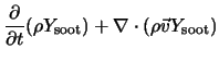
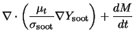
In the one-step Khan and Greeves model [ 162], ANSYS FLUENT solves a single transport equation for the soot mass fraction:
| where | ||
 |
= soot mass fraction | |
 |
= turbulent Prandtl number for soot transport | |
 |
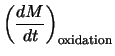
= net rate of soot generation (kg/m
 -s) -s) |
 , the net rate of soot generation, is the balance of soot formation,
 , and soot combustion,
 :
:
 |
(13.3-2) |
The rate of soot formation is given by a simple empirical rate expression:
| where | ||
 |
= soot formation constant (kg/N-m-s) | |
 |
= fuel partial pressure (Pa) | |
 |
= equivalence ratio | |
 |
= equivalence ratio exponent | |
 |
= activation temperature (K) |
The rate of soot combustion is the minimum of two rate expressions [ 216]:
The two rates are computed as
and
| where | ||
 |
= constant in the Magnussen model | |
 , ,
 |
= mass fractions of oxidizer and fuel | |
 , ,
 |
= mass stoichiometries for soot and fuel combustion |
The default constants for the one-step model are valid for a wide range of hydrocarbon fuels.
The Two-Step Soot Formation Model
The two-step Tesner model [ 349] predicts the generation of radical nuclei and then computes the formation of soot on these nuclei. ANSYS FLUENT thus solves transport equations for two scalar quantities: the soot mass fraction (Equation 13.3-1) and the normalized radical nuclei concentration:
| where | ||
 |
= normalized radical nuclei concentration (particles
 /kg) /kg) | |
 |
= turbulent Prandtl number for nuclei transport | |
 |
= normalized net rate of nuclei generation (particles
 /m /m
 -s) -s) |
In these transport equations, the rates of nuclei and soot generation are the net rates, involving a balance between formation and combustion.
Soot Generation Rate
The two-step model computes the net rate of soot generation,
 , in the same way as the one-step model, as a balance of soot formation and soot combustion:
 |
(13.3-8) |
In the two-step model, however, the rate of soot formation,
 , depends on the concentration of radical nuclei,
 :
:
| where | ||
 |
= mean mass of soot particle (kg/particle) | |
 |
= concentration of soot particles (particles/m
 ) ) | |
 |
= radical nuclei concentration =
 (particles/m (particles/m
 ) ) | |
 |
= empirical constant (s
 ) ) | |
 |
= empirical constant (m
 /particle-s) /particle-s) |
The rate of soot combustion,
 , is computed in the same way as for the one-step model, using Equations
13.3-4-
13.3-6.
, is computed in the same way as for the one-step model, using Equations
13.3-4-
13.3-6.
The default constants for the two-step model are for combustion of acetylene (C
 H
H
 ). According to Ahmad et al. [
2], these values should be modified for other fuels, since the sooting characteristics of acetylene are known to be different from those of saturated hydrocarbon fuels.
). According to Ahmad et al. [
2], these values should be modified for other fuels, since the sooting characteristics of acetylene are known to be different from those of saturated hydrocarbon fuels.
Nuclei Generation Rate
The net rate of nuclei generation in the two-step model is given by the balance of the nuclei formation rate and the nuclei combustion rate:
 |
(13.3-10) |
| where | ||
 |
= rate of nuclei formation (particles
 /m /m
 -s) -s) | |
 |
= rate of nuclei combustion (particles
 /m /m
 -s) -s) |
The rate of nuclei formation,
 , depends on a spontaneous formation and branching process, described by
| where | ||
 |
= normalized nuclei concentration (
 ) ) | |
 |
=
 | |
 |
= pre-exponential rate constant (particles/kg-s) | |
 |
= fuel concentration (kg/m
 ) ) | |
 |
= linear branching
 termination coefficient (s termination coefficient (s
 ) ) | |
 |
= linear termination on soot particles (m
 /particle-s) /particle-s) |
Note that the branching term,
 , in Equation
13.3-11 is included only when the kinetic rate,
, in Equation
13.3-11 is included only when the kinetic rate,
 , is greater than the limiting formation rate (10
 particles/m
 -s, by default).
The rate of nuclei combustion is assumed to be proportional to the rate of soot combustion:
 |
(13.3-13) |
where the soot combustion rate,
 , is given by Equation
13.3-4.
, is given by Equation
13.3-4.
The Moss-Brookes Model
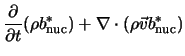
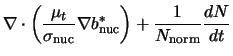
The Moss-Brookes model solves transport equations for normalized radical nuclei concentration
 and soot mass fraction
 :
:
| where | ||
 |
= soot mass fraction | |
 |
= soot mass concentration (kg/m
 ) ) | |
 |
= normalized radical nuclei concentration (particles
 /kg) = /kg) =
 | |
 |
= soot particle number density (particles/m
 ) ) | |
 |
= 10
 particles particles |
The instantaneous production rate of soot particles, subject to nucleation from the gas phase and coagulation in the free molecular regime, is given by
where
 ,
,
 and
and
 are model constants. Here,
 (= 6.022045x10
 kmol
kmol
 ) is the Avogadro number and
 is the mole fraction of soot precursor (for methane, the precursor is assumed to be acetylene, whereas for kerosene it is a combination of acetylene and benzene). The mass density of soot,
 , is assumed to be 1800 kg/m
 and
and
 is the mean diameter of a soot particle. The nucleation rate for soot particles is taken to be proportional to the local acetylene concentration for methane. The activation temperature
 for the nucleation reaction is that proposed by Lindstedt [
199].
for the nucleation reaction is that proposed by Lindstedt [
199].
The source term for soot mass concentration is modeled by the expression
where
 ,
,
 ,
,
 ,
,
 , and
, and
 are additional model constants. The constant
 (= 144 kg/kgmol) is the mass of an incipient soot particle, here taken to consist of 12 carbon atoms. Even though the model is not found to be sensitive to this assumption, a nonzero initial mass is needed to begin the process of surface growth. Here,
 is the mole fraction of the participating surface growth species. For paraffinic fuels, soot particles have been found to grow primarily by the addition of gaseous species at their surfaces, particularly acetylene that has been found in abundance in the sooting regions of laminar methane diffusion flames.
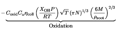
The model assumes that the hydroxyl radical is the dominant oxidizing agent in methane/air diffusion flames and that the surface-specific oxidation rate of soot by the OH radical may be formulated according to the model proposed by Fenimore and Jones [
93]. Assuming a collision efficiency (
 ) of 0.04, the oxidation rate may be written as (Equation
13.3-17.
) of 0.04, the oxidation rate may be written as (Equation
13.3-17.
The process of determination of the exponents
 ,
,
 , and
, and
 are explained in detail by Brookes and Moss [
39]. The constants
are explained in detail by Brookes and Moss [
39]. The constants
 and
and
 are determined through numerical modeling of a laminar flame for which experimental data exists.
The set of constants proposed by Brookes and Moss for methane flames are given below:
 |
= 54 s
 (model constant for soot inception rate) (model constant for soot inception rate) | |
 |
= 21000 K (activation temperature of soot inception) | |
 |
= 1.0 (model constant for coagulation rate) | |
 |
= 11700 kg.m.kmol
 .s .s
 (surface growth rate scaling factor) (surface growth rate scaling factor) | |
 |
= 12100 K (activation temperature of surface growth rate) | |
 |
= 105.8125 kg.m.kmol
 .K .K
 .s .s
 (oxidation model constant) (oxidation model constant) | |
 |
= 0.04 (collisional efficiency parameter) | |
 |
= 0.015 (oxidation rate scaling parameter) |
Note that the implementation of the Moss-Brookes model in
ANSYS FLUENT uses the values listed above, except for
 which is set to unity by default.
The closure for the mean soot source terms in the above equations was also described in detail by Brookes and Moss [ 39]. The uncorrelated closure is the preferred option for a tractable solution of the above transport equations.
Moss et al. [
239] have shown the above model applied to kerosene flames by modifying only the soot precursor species (in the original model the precursor was acetylene, whereas for kerosene flames the precursor was assumed to be a combination of both acetylene and benzene) and by setting the value of oxidation scaling parameter
 to unity. A good comparison against the experimental measurements for the lower pressure (7 bar) conditions was observed. The predictions of soot formation within methane flames have shown the Brooks and Moss [
39] model to be superior compared with the standard Tesner et al. [
349] formulation.
to unity. A good comparison against the experimental measurements for the lower pressure (7 bar) conditions was observed. The predictions of soot formation within methane flames have shown the Brooks and Moss [
39] model to be superior compared with the standard Tesner et al. [
349] formulation.
The Coal-Derived Soot Extension (Beta Feature)
The present implementation provides an extension to the Moss-Brookes soot model that accounts for coal-derived soot, based on the work of Brown [ 41]. This extension includes an additional transport equation for the tar evolved during coal devolatilization. The Moss-Brookes model assumes that the physical properties of tar is similar to those of volatiles, such that the combined effect of volatile and tar on the gas phase flame simulation may be replaced by a single volatile stream (consisting of volatile and tar). In reality, however, this may not be the case, and so the coal-derived soot extension allows you to treat the tar contribution similar to that of volatiles.
The following set of paths was assumed for the coal-derived soot formation [ 214] (see Figure 13.3.1).
Nucleation is assumed to be the first step in formation of soot in most light gas flames, and acetylene is understood to be the major species involved. In heavier gas flames, benzene and other polycyclic aromatic hydrocarbons (PAHs) may contribute to soot formation as well. Soot formation in coal flames is thought to occur as tars or the higher molecular weight hydrocarbons given off during devolatilization combine and condense to form soot particles. This is a different mechanism to that of soot formation from gaseous fuels. The related source term for each path is given as follows:
where
 is equal to 10
 particles,
 is Avogadro's Number, and
 is the molecular weight of the soot particle. The remaining terms in the previous overall source expressions are defined as follows:
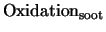
The soot oxidation term (
 ) is similar to that shown in Equation
13.3-17 in the Moss-Brookes soot model theory (Fenimore-Jones or Lee oxidation model). Soot density (
) is similar to that shown in Equation
13.3-17 in the Moss-Brookes soot model theory (Fenimore-Jones or Lee oxidation model). Soot density (
 ) is assumed to be 1950 kg/m
 and the collision constant
 is set to 3.0.
 (= 12 kg/kgmol) is the molecular weight of carbon and
 (= 1.3806503e-23 J/K) is the Boltzmann constant. An incipient soot particle is assumed to consist of 9e+04 carbon atoms, thus making
 = 108e+04 kg/kgmol.
 is the normalized radical nuclei concentration (i.e., the number of particles
 /kg). Since the coal-derived soot particles are large, the turbulent Schmidt number used in the transport equations for soot mass fraction and the normalized number density must be modified to account for the particle size. A value of 700 for the turbulent Schmidt number is suggested for soot mass fraction and nuclei transport.
The term
 is the tar release rate from coal (kg/m
 -s) and comes from the coal particle source computations of the discrete phase model. It is assumed that the mass fraction of tar in coal volatiles is in the range 0.3-0.5, and therefore the
 term is related to the volatile source term via the tar mass fraction in volatiles. One of the main assumptions of this implementation is that tar may be decoupled from the flow field computations, since tar is a fraction of volatiles and volatile transport is fully coupled with the flow field.
The values used for the pre-exponential constant
 and the activation energy
 in Equations
13.3-22-
13.3-24 are listed in Table
13.3.1.
in Equations
13.3-22-
13.3-24 are listed in Table
13.3.1.
The Moss-Brookes-Hall Model
Since the Moss-Brookes model was mainly developed and validated for methane flames, a further extension for higher hydrocarbon fuels called the Moss-Brookes-Hall model was also included in the present ANSYS FLUENT implementation. Here, the extended version is a model reported by Wen et al. [ 374] based on model extensions proposed by Hall et al. [ 120] and an oxidation model proposed by Lee et al. [ 184]. The work of Hall [ 120] is based on a soot inception rate due to two-ringed and three-ringed aromatics, as opposed to the Moss-Brookes assumption of a soot inception due to acetylene or benzene (for higher hydrocarbons).
Hall et al. [
120] proposed a soot inception rate based on the formation rates of two-ringed and three-ringed aromatics (C
 H
H
 and C
and C
 H
H
 ), from acetylene (C
 H
H
 ), benzene (C
 H
H
 ), and the phenyl radical (C
 H
H
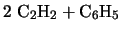
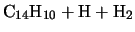
 ) based on the following mechanisms:
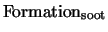
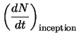
Based on their laminar methane flame data, the inception rate of soot particles was given to be eight times the formation rate of species C
 H
H
 and C
and C
 H
H
 , as shown by
where
 = 127x10
 s
s
 ,
,
 = 178x10
 s
s
 ,
,
 = 4378 K, and
 = 6390 K as determined by Hall et al. [
120]. In their model, the mass of an incipient soot particle was assumed to be 1200 kg/kgmol (corresponding to 100 carbon atoms, as opposed to 12 carbon atoms used by Brookes and Moss [
39]). The mass density of soot was assumed to be 2000 kg/m
= 6390 K as determined by Hall et al. [
120]. In their model, the mass of an incipient soot particle was assumed to be 1200 kg/kgmol (corresponding to 100 carbon atoms, as opposed to 12 carbon atoms used by Brookes and Moss [
39]). The mass density of soot was assumed to be 2000 kg/m
 , which is also slightly different from the value used by Brookes and Moss. [
39]
, which is also slightly different from the value used by Brookes and Moss. [
39]
Both the coagulation term and the surface growth term were formulated similar to those used by Brookes and Moss [
39] with a slight modification to the constant
 so that the value is 9000.6 kg.m.kmol
 .s
.s
 (based on the model developed by Lindstedt [
200]).
(based on the model developed by Lindstedt [
200]).
For the soot oxidation term, oxidation due to O
 (based on measurements and model based on Lee et al. [
184]) was added, in addition to the soot oxidation due to the hydroxyl radical. By assuming that the kinetics of surface reactions is the limiting mechanism and that the particles are small enough to neglect the diffusion effect on the soot oxidation, they derived the specific rate of soot oxidation by molecular oxygen. Therefore the full soot oxidation term, including that due to hydroxyl radical, is of the form
(based on measurements and model based on Lee et al. [
184]) was added, in addition to the soot oxidation due to the hydroxyl radical. By assuming that the kinetics of surface reactions is the limiting mechanism and that the particles are small enough to neglect the diffusion effect on the soot oxidation, they derived the specific rate of soot oxidation by molecular oxygen. Therefore the full soot oxidation term, including that due to hydroxyl radical, is of the form
Here, the collision efficiency is assumed to be 0.13 (compared to 0.04 used by Brookes and Moss) and the oxidation rate scaling parameter is assumed to be unity. The model constants used are as follows:
| where | ||
 |
= 105.81 kg.m.kmol
 .K .K
 .s .s
 (same as that used by Brookes and (same as that used by Brookes and | |
| Moss) | ||
 |
= 8903.51 kg.m.kmol
 .K .K
 .s .s
 | |
 |
= 19778 K |
Soot Formation in Turbulent Flows
The kinetic mechanisms of soot formation and destruction for the Moss-Brookes model and the Hall extension are obtained from laboratory experiments in a similar fashion to the NOx model. In any practical combustion system, however, the flow is highly turbulent. The turbulent mixing process results in temporal fluctuations in temperature and species concentration that will influence the characteristics of the flame.
The relationships among soot formation rate, temperature, and species concentration are highly nonlinear. Hence, if time-averaged composition and temperature are employed in any model to predict the mean soot formation rate, significant errors will result. Temperature and composition fluctuations must be taken into account by considering the probability density functions which describe the time variation.
The Turbulence-Chemistry Interaction Model
In turbulent combustion calculations, ANSYS FLUENT solves the density-weighted time-averaged Navier-Stokes equations for temperature, velocity, and species concentrations or mean mixture fraction and variance. To calculate soot concentration for the Moss-Brookes model and the Hall extension, a time-averaged soot formation rate must be computed at each point in the domain using the averaged flow-field information.
The PDF Approach
The PDF method has proven very useful in the theoretical description of turbulent flow [ 149]. In the ANSYS FLUENT Moss-Brookes model and the Hall extension, a single- or joint-variable PDF in terms of a normalized temperature, species mass fraction, or the combination of both is used to predict the soot formation. If the non-premixed combustion model is used to model combustion, then a one- or two-variable PDF in terms of mixture fraction(s) is also available. The mean values of the independent variables needed for the PDF construction are obtained from the solution of the transport equations.
The Mean Reaction Rate
The mean turbulent reaction rate described in Section 13.1.9 for the NOx model also applies to the Moss-Brookes model and the Hall extension. The PDF is used for weighting against the instantaneous rates of production of soot and subsequent integration over suitable ranges to obtain the mean turbulent reaction rate as described in Equations 13.1-104 and 13.1-105 for NOx.
The PDF Options
As is the case with the NOx model,
 can be calculated as either a two-moment beta function or as a clipped Gaussian function, as appropriate for combustion calculations [
123,
231]. Equations
13.1-107 -
13.1-111 apply to the Moss-Brookes model and Hall extension as well, with the variance
can be calculated as either a two-moment beta function or as a clipped Gaussian function, as appropriate for combustion calculations [
123,
231]. Equations
13.1-107 -
13.1-111 apply to the Moss-Brookes model and Hall extension as well, with the variance
 computed by solving a transport equation during the combustion calculation stage, using Equation
13.1-112 or Equation
13.1-113.
computed by solving a transport equation during the combustion calculation stage, using Equation
13.1-112 or Equation
13.1-113.
The Effect of Soot on the Radiation Absorption Coefficient
A description of the modeling of soot-radiation interaction is provided in Section 5.3.8.
Previous:
13.3.1 Overview and Limitations


![{\cal R}_{\rm soot, comb} = \min [{\cal R}_1, \; {\cal R}_2 ]](img5238.gif)











![$\displaystyle \underbrace{M_{\rm P} C_{\alpha} \left(\frac{X_{\rm prec} P}{R T... ... \frac{6 M}{\rho_{\rm soot}} \right)^{2/3} \right]^{n}}_{\mbox{Surface Growth}}$](img5331.gif)










 (kJ/kgmol)
 /kg-s)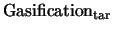





![$\displaystyle 8 C_{\alpha,1} \frac{N_{\rm A}}{M_{\rm P}} \left[ \rho^{2} \left(... ...}Y_{H_{2}}} \right] \exp \left\{-\frac{T_{\alpha, 1}}{T} \right\} \hspace{.8in}$](img5417.gif)
![$\displaystyle + 8 C_{\alpha, 2} \frac{N_{\rm A}}{M_{\rm P}} \left[ \rho^{2} \fr... ..._{C_{6}H_{5}}Y_{H_{2}}} \right] \exp \left\{ - \frac{T_{\alpha, 2}}{T} \right\}$](img5418.gif)