![[ANSYS, Inc. Logo]](fluentlogo.gif)


|
|
|
 -
-
 Model
Model
Overview
The realizable
 -
-
 model [
313] is a relatively recent development and differs from the standard
model [
313] is a relatively recent development and differs from the standard
 -
-
 model in two important ways:
 -
-
 model contains a new formulation for the turbulent viscosity.
 , has been derived from an exact equation for the transport of the mean-square vorticity fluctuation.
 The term "realizable'' means that the model satisfies certain mathematical constraints on the Reynolds stresses, consistent with the physics of turbulent flows. Neither the standard
 -
-
 model nor the RNG
 -
-
 model is realizable.
An immediate benefit of the realizable
 -
-
 model is that it more accurately predicts the spreading rate of both planar and round jets. It is also likely to provide superior performance for flows involving rotation, boundary layers under strong adverse pressure gradients, separation, and recirculation.
To understand the mathematics behind the realizable
 -
-
 model, consider combining the Boussinesq relationship (Equation
4.2-5) and the eddy viscosity definition (Equation
4.4-3) to obtain the following expression for the normal Reynolds stress in an incompressible strained mean flow:
model, consider combining the Boussinesq relationship (Equation
4.2-5) and the eddy viscosity definition (Equation
4.4-3) to obtain the following expression for the normal Reynolds stress in an incompressible strained mean flow:
Using Equation
4.4-3 for
 , one obtains the result that the normal stress,
 , which by definition is a positive quantity, becomes negative, i.e., "non-realizable'', when the strain is large enough to satisfy
Similarly, it can also be shown that the Schwarz inequality for shear stresses (
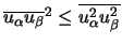 ; no summation over
 and
and
 ) can be violated when the mean strain rate is large. The most straightforward way to ensure the realizability (positivity of normal stresses and Schwarz inequality for shear stresses) is to make
 variable by sensitizing it to the mean flow (mean deformation) and the turbulence (
 ,
,
 ). The notion of variable
 is suggested by many modelers including Reynolds [
291], and is well substantiated by experimental evidence. For example,
is suggested by many modelers including Reynolds [
291], and is well substantiated by experimental evidence. For example,
 is found to be around 0.09 in the inertial sublayer of equilibrium boundary layers, and 0.05 in a strong homogeneous shear flow.
Both the realizable and RNG
 -
-
 models have shown substantial improvements over the standard
 -
-
 model where the flow features include strong streamline curvature, vortices, and rotation.
Since the model is still relatively new, it is not clear in exactly which instances the realizable
model where the flow features include strong streamline curvature, vortices, and rotation.
Since the model is still relatively new, it is not clear in exactly which instances the realizable
 -
-
 model consistently outperforms the RNG model. However, initial studies have shown that the realizable model provides the best performance of all the
 -
-
 model versions for several validations of separated flows and flows with complex secondary flow features.
One of the weaknesses of the standard
 -
-
 model or other traditional
 -
-
 models lies with the modeled equation for the dissipation rate (
 ). The well-known round-jet anomaly (named based on the finding that the spreading rate in planar jets is predicted reasonably well, but prediction of the spreading rate for axisymmetric jets is unexpectedly poor) is considered to be mainly due to the modeled dissipation equation.
The realizable
 -
-
 model proposed by Shih et al. [
313] was intended to address these deficiencies of traditional
model proposed by Shih et al. [
313] was intended to address these deficiencies of traditional
 -
-
 models by adopting the following:
 originally proposed by Reynolds [
291].
originally proposed by Reynolds [
291].
 ) based on the dynamic equation of the mean-square vorticity fluctuation.
 One limitation of the realizable
 -
-
 model is that it produces non-physical turbulent viscosities in situations when the computational domain contains both rotating and stationary fluid zones (e.g., multiple reference frames, rotating sliding meshes). This is due to the fact that the realizable
 -
-
 model includes the effects of mean rotation in the definition of the turbulent viscosity (see Equations
4.4-17-
4.4-19). This extra rotation effect has been tested on single rotating reference frame systems and showed superior behavior over the standard
model includes the effects of mean rotation in the definition of the turbulent viscosity (see Equations
4.4-17-
4.4-19). This extra rotation effect has been tested on single rotating reference frame systems and showed superior behavior over the standard
 -
-
 model. However, due to the nature of this modification, its application to multiple reference frame systems should be taken with some caution. See Section
4.4.3 for information about how to include or exclude this term from the model.
model. However, due to the nature of this modification, its application to multiple reference frame systems should be taken with some caution. See Section
4.4.3 for information about how to include or exclude this term from the model.
Transport Equations for the Realizable
 -
-
 Model
Model
The modeled transport equations for
 and
and
 in the realizable
 -
-
 model are
and
where
![C_1 = \max\left[0.43, \frac{\eta}{\eta + 5}\right] , \;\;\;\;... ...a = S \frac{k}{\epsilon}, \;\;\;\;\; S =\sqrt{2 S_{ij} S_{ij}}](img896.gif)
In these equations,
 represents the generation of turbulence kinetic energy due to the mean velocity gradients, calculated as described in Section
4.4.4.
represents the generation of turbulence kinetic energy due to the mean velocity gradients, calculated as described in Section
4.4.4.
 is the generation of turbulence kinetic energy due to buoyancy, calculated as described in Section
4.4.5.
is the generation of turbulence kinetic energy due to buoyancy, calculated as described in Section
4.4.5.
 represents the contribution of the fluctuating dilatation in compressible turbulence to the overall dissipation rate, calculated as described in Section
4.4.6.
represents the contribution of the fluctuating dilatation in compressible turbulence to the overall dissipation rate, calculated as described in Section
4.4.6.
 and
and
 are constants.
 and
and
 are the turbulent Prandtl numbers for
 and
and
 , respectively.
 and
and
 are user-defined source terms.
Note that the
 equation (Equation
4.4-15) is the same as that in the standard
equation (Equation
4.4-15) is the same as that in the standard
 -
-
 model (Equation
4.4-1) and the RNG
model (Equation
4.4-1) and the RNG
 -
-
 model (Equation
4.4-4), except for the model constants. However, the form of the
model (Equation
4.4-4), except for the model constants. However, the form of the
 equation is quite different from those in the standard and RNG-based
 -
-
 models (Equations
4.4-2 and
4.4-5). One of the noteworthy features is that the production term in the
models (Equations
4.4-2 and
4.4-5). One of the noteworthy features is that the production term in the
 equation (the second term on the right-hand side of Equation
4.4-16) does not involve the production of
equation (the second term on the right-hand side of Equation
4.4-16) does not involve the production of
 ; i.e., it does not contain the same
 term as the other
 -
-
 models. It is believed that the present form better represents the spectral energy transfer. Another desirable feature is that the destruction term (the next to last term on the right-hand side of Equation
4.4-16) does not have any singularity; i.e., its denominator never vanishes, even if
models. It is believed that the present form better represents the spectral energy transfer. Another desirable feature is that the destruction term (the next to last term on the right-hand side of Equation
4.4-16) does not have any singularity; i.e., its denominator never vanishes, even if
 vanishes or becomes smaller than zero. This feature is contrasted with traditional
 -
-
 models, which have a singularity due to
 in the denominator.
This model has been extensively validated for a wide range of flows [
167,
313], including rotating homogeneous shear flows, free flows including jets and mixing layers, channel and boundary layer flows, and separated flows. For all these cases, the performance of the model has been found to be substantially better than that of the standard
 -
-
 model. Especially noteworthy is the fact that the realizable
 -
-
 model resolves the round-jet anomaly; i.e., it predicts the spreading rate for axisymmetric jets as well as that for planar jets.
Modeling the Turbulent Viscosity
As in other
 -
-
 models, the eddy viscosity is computed from
The difference between the realizable
 -
-
 model and the standard and RNG
 -
-
 models is that
 is no longer constant. It is computed from
where
and
 |
 |
 |
|
 |
 |
 |
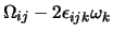
where
 is the mean rate-of-rotation tensor viewed in a rotating reference frame with the angular velocity
 . The model constants
 and
and
 are given by

where

It can be seen that
 is a function of the mean strain and rotation rates, the angular velocity of the system rotation, and the turbulence fields (
 and
and
 ).
).
 in Equation
4.4-17 can be shown to recover the standard value of 0.09 for an inertial sublayer in an equilibrium boundary layer.
in Equation
4.4-17 can be shown to recover the standard value of 0.09 for an inertial sublayer in an equilibrium boundary layer.
Model Constants
The model constants
 ,
,
 , and
, and
 have been established to ensure that the model performs well for certain canonical flows. The model constants are

Previous:
4.4.2 RNG - Model


![\frac{\partial}{\partial t} (\rho k) + \frac{\partial}{\part... ...\partial x_j} \right ] + G_k + G_b - \rho \epsilon - Y_M + S_k](img894.gif)





 is, by default, not included in the calculation of
 . This is an extra rotation term that is not compatible with cases involving sliding meshes or multiple reference frames. If you want to include this term in the model, you can enable it by using the
define/models/viscous/turbulence-expert/rke-cmu-rotation-term? text command and entering
yes at the prompt.
. This is an extra rotation term that is not compatible with cases involving sliding meshes or multiple reference frames. If you want to include this term in the model, you can enable it by using the
define/models/viscous/turbulence-expert/rke-cmu-rotation-term? text command and entering
yes at the prompt.