29.10.5 Generating Averaged XY Plots of Turbomachinery Solution Data

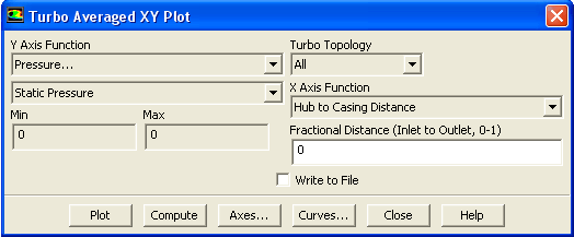
When comparing numerical solutions of turbomachinery problems to experimental data, it is often useful to plot circumferentially averaged quantities in the spanwise and meridional directions. This section describes how to do this in ANSYS FLUENT.

Steps for Generating Turbo Averaged XY Plots

To create an XY plot of circumferentially averaged solution data, you will use the Turbo Averaged XY Plot dialog box (Figure  29.10.9).

Turbo $\rightarrow$ Averaged XY Plot...

Figure 29.10.9: The Turbo Averaged XY Plot Dialog Box

The basic steps for generating a turbo averaged XY plot are as follows:

1.   Select the variable or function to be plotted in the Y Axis Function drop-down list. First select the desired category in the upper list; you may then select a related quantity in the lower list. (See Section  29.10.7 for a list of turbomachinery-specific variables, and see Chapter  31 for an explanation of the variables in the list.)

2.   Select All or a specific predefined turbomachinery topology from the Turbo Topology drop-down list.

3.   Select the variable or function to be plotted in the X Axis Function drop-down list. The choices are Hub to Casing Distance and Meridional Distance.

4.   Specify the desired value in the Fractional Distance field. The definition of the fractional distance depends on your selection of X Axis Function:

• If you selected Hub to Casing Distance, the fractional distance is Inlet to Outlet.

• If you selected Meridional Distance, the fractional distance is Hub to Casing.

5.   (optional) Modify the attributes of the axes or curves as described in Sections  29.9.9 and 29.9.10.

6.   Click the Plot button to generate the XY plot in the active graphics window.

Note that you can use any of the mouse buttons to annotate the XY plot (see Section  29.2.4).

If you wish to write the XY data to a file, follow these steps instead of Step 5 above:

1.   Turn on the Write to File option. The Plot button will change to the Write... button.

2.   Click Write....

3.   In the resulting Select File dialog box (see Section  2.1.6), specify a name for the plot file and save it.