29.10.2 Generating Reports of Turbomachinery Data

Once you have defined your turbomachinery topologies, as described in Section  29.10.1, you can report a number of turbomachinery quantities, including mass flow, swirl number, torque, and efficiencies.

To report turbomachinery quantities in ANSYS FLUENT, you will use the Turbo Report dialog box (Figure  29.10.3).

Turbo $\rightarrow$ Report...

Figure 29.10.3: The Turbo Report Dialog Box

The procedure for using this dialog box is as follows:

1.   Under Averages, specify whether you want to report Mass-Weighted or Area-Weighted averages.

2.   Under Turbo Topology, specify a predefined turbomachinery topology from the drop-down list.

3.   Click Compute. ANSYS FLUENT will compute the turbomachinery quantities as described below, and display their values.

4.   If you want to save the reported values to a file, click Write... and specify a name for the file in the resulting Select File dialog box (see Section  2.1.6).

Computing Turbomachinery Quantities

Mass Flow

The mass flow rate through a surface is defined as follows:

where $A$ is the area of the inlet or outlet, $\vec{v}$ is the velocity vector, $\rho$ is the fluid density, and $\hat{n}$ is a unit vector normal to the surface.

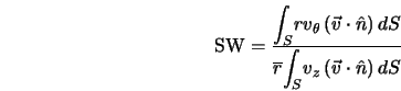
Swirl Number

The swirl number is defined as follows:

where $r$ is the radial coordinate (specifically, the radial distance from the axis of rotation), $v_{\theta}$ is the tangential velocity, $\vec{v}$ is the velocity vector, $\hat{n}$ is a unit vector normal to the surface, $S$ denotes the inlet or outlet, and

Average Total Pressure

The area-averaged total pressure is defined as follows:

where $p_t$ is the total pressure and $A$ is the area of the inlet or outlet.

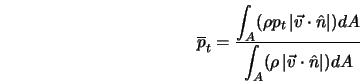
The mass-averaged total pressure is defined as follows:

where $p_t$ is the total pressure, $A$ is the area of the inlet or outlet, $\vec{v}$ is the velocity vector, $\rho$ is the fluid density, and $\hat{n}$ is a unit vector normal to the surface.

Average Total Temperature

The area-averaged total temperature is defined as follows:

where $T_t$ is the total temperature and $A$ is the area of the inlet or outlet.

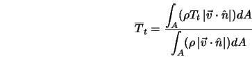
The mass-averaged total temperature is defined as follows:

where $T_t$ is the total temperature, $A$ is the area of the inlet or outlet, $\vec{v}$ is the velocity vector, $\rho$ is the fluid density, and $\hat{n}$ is a unit vector normal to the surface.

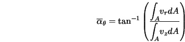
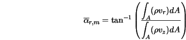
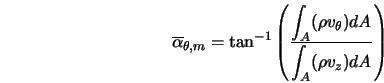
Average Flow Angles

The area-averaged flow angles are defined as follows:

in the radial direction, and

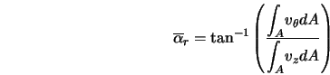
in the tangential direction, where $v_z$, $v_r$, and $v_{\theta}$ represent the axial, radial, and tangential velocities, respectively.

The mass-averaged flow angles are defined as follows:

in the radial direction, and

in the tangential direction.

Passage Loss Coefficient

The engineering loss coefficient is defined as follows:

where $\overline{p}_{t,i}$ is the mass-averaged total pressure at the inlet, $\overline{p}_{t,o}$ is the mass-averaged total pressure at the outlet, $\rho$ is the density of the fluid, and $\overline{v}_i$ is the mass-averaged velocity magnitude at the inlet.

The normalized loss coefficient is defined as follows:

where $\overline{p}_{s,o}$ is the mass-averaged static pressure at the outlet.

Axial Force

The axial force on the rotating parts is defined as follows:

where $S$ represents the surfaces comprising all rotating parts, $\overline{\overline{\tau}}$ is the total stress tensor (pressure and viscous stresses), $\hat{n}$ is a unit vector normal to the surface, and $\hat{a}$ is a unit vector parallel to the axis of rotation.

Torque

The torque on the rotating parts is defined as follows:

where $S$ represents the surfaces comprising all rotating parts, $\overline{\overline{\tau}}$ is the total stress tensor, $\hat{n}$ is a unit vector normal to the surface, $\vec{r}$ is the position vector, and $\hat{a}$ is a unit vector parallel to the axis of rotation.

Efficiencies for Pumps and Compressors

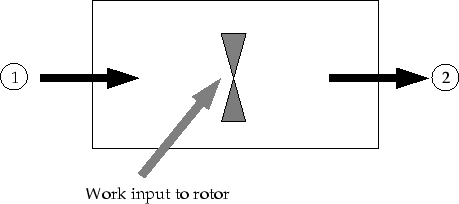
The definitions of the efficiencies for compressible and incompressible flows in pumps and compressors are described in this section. Efficiencies for turbines are described later in this section. Consider a pumping or compression device operating between states 1 and 2 as illustrated in Figure  29.10.4. Work input to the device is required to achieve a specified compression of the working fluid.

Figure 29.10.4: Pump or Compressor

Assuming that the processes are steady state, steady flow, and that the mass flow rates are equal at the inlet and outlet of the device (no film cooling, bleed air removal, etc.), the efficiencies for incompressible and compressible flows are as described below.

Incompressible Flows

For devices such as liquid pumps and fans at low speeds, the working fluid can be treated as incompressible. The efficiency of a pumping process with an incompressible working fluid is defined as the ratio of the head rise achieved by the fluid to the power supplied to the rotor/impeller. This can be expressed as follows:

where
	$Q$	=	volumetric flow rate
	$p_t$	=	total pressure
	$T$	=	net torque acting on the rotor/impeller
	$\omega$	=	rotational speed

This definition is sometimes called the "hydraulic efficiency''. Often, other efficiencies are included to account for flow leakage (volumetric efficiency) and mechanical losses along the transmission system between the rotor and the machine providing the power for the rotor/impeller (mechanical efficiency). Incorporating these losses then yields a total efficiency for the system.

Compressible Flows

For gas compressors that operate at high speeds and high pressure ratios, the compressibility of the working fluid must be taken into account. The efficiency of a compression process with a compressible working fluid is defined as the ratio of the work required for an ideal (reversible) compression process to the actual work input. This assumes the compression process occurs between states 1 and 2 for a given pressure ratio. In most cases, the pressure ratio is the total pressure at state 2 divided by the total pressure at state 1. If the process is also adiabatic, then the ideal state at 2 is the isentropic state.

From the foregoing definition, the efficiency for an adiabatic compression process can be written as

where
	$h_{t1}$	=	total enthalpy at 1
	$h_{t2}$	=	actual total enthalpy at 2
	$h_{t2,i}$	=	isentropic total enthalpy at 2

If the specific heat is constant, Equation  29.10-17 can also be expressed as

where
	$T_{t1}$	=	total temperature at 1
	$T_{t2}$	=	actual total temperature at 2
	$T_{t2,i}$	=	isentropic total temperature at 2

Using the isentropic relation

where $\gamma$ is the ratio of specific heats specified in the Reference Values task page.

The efficiency can be written in the compact form

Note that this definition requires data only for the actual states 1 and 2.

Compressor designers also make use of the polytropic efficiency when comparing one compressor with another. The polytropic efficiency is defined as follows:

Efficiencies for Turbines

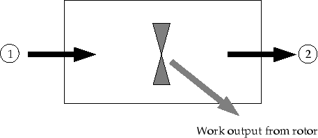
Consider a turbine operating between states 1 and 2 in Figure  29.10.5. Work is extracted from the working fluid as it expands through the turbine. Assuming that the processes are steady state, steady flow, and that the mass flow rates are equal at the inlet and outlet of the device (no film cooling, bleed air removal, etc.), turbine efficiencies for incompressible and compressible flows are as described below.

Figure 29.10.5: Turbine

Incompressible Flows

The efficiency of a turbine with an incompressible working fluid is defined as the ratio of the work delivered to the rotor to the energy available from the fluid stream. This ratio can be expressed as follows:

where
	$Q$	=	volumetric flow rate
	$p_t$	=	total pressure
	$T$	=	net torque acting on the rotor/impeller
	$\omega$	=	rotational speed

Note the similarity between this definition and the definition of incompressible compression efficiency (Equation  29.10-16). As with hydraulic pumps and compressors, other efficiencies (e.g., volumetric and mechanical efficiencies) can be defined to account for other losses in the system.

Compressible Flows

For high-speed gas turbines operating at large expansion pressure ratios, compressibility must be accounted for. The efficiency of an expansion process with a compressible working fluid is defined as the ratio of the actual work extracted from the fluid to the work extracted from an ideal (reversible) process. This assumes that the expansion process occurs between states 1 and 2 for a given pressure ratio. In contrast to the compression process, the pressure ratio for expansion is the total pressure at state 1 divided by the total pressure at state 2. If the process is also adiabatic, then the ideal state at 2 is the isentropic state.

From the foregoing definition, the efficiency for an adiabatic expansion process through a turbine can be written as

where
	$h_{t1}$	=	total enthalpy at 1
	$h_{t2}$	=	actual total enthalpy at 2
	$h_{t2,i}$	=	isentropic total enthalpy at 2

If the specific heat is constant, Equation  29.10-23 can also be expressed as

where
	$T_{t1}$	=	total temperature at 1
	$T_{t2}$	=	actual total temperature at 2
	$T_{t2,i}$	=	isentropic total temperature at 2

Using the isentropic relation

the expansion efficiency can be written in the compact form

Note that this definition requires data only for the actual states 1 and 2.

As with compressors, one may also define a polytropic efficiency for turbines. The polytropic efficiency is defined as follows: