21.2.1 Using the SOx Model

When the sulfur content in the fuel is low, SOx concentrations that are generated in combustion generally have minimal influence on the predicted flow field, temperature, and major combustion product concentrations. The most efficient way to use the SOx model is as a postprocessor to the main combustion calculation. However, if the sulfur content is high, then SOx formation should be coupled with the gas phase combustion process rather than treating it as a postprocessing step.

The procedure for activating and setting up the model for a decoupled solution is as follows:

1.   Calculate your combustion problem using ANSYS FLUENT.

The premixed combustion model is not compatible with the SOx model.

2.   Enable the SOx model, define the fuel streams, and set the appropriate parameters, as described in this section.

Models SOx Edit...

3.   Define the boundary conditions for $\rm {SO}_2$ and $\rm {H}_{2}{\rm {S}}$ (and $\rm {SO}_3$, SH, or SO if necessary) at flow inlets.

Boundary Conditions

4.   In the Equations dialog box, turn off the solution of all variables except species $\rm {SO}_2$ and $\rm {H}_{2}{\rm {S}}$ (and $\rm {SO}_3$, SH, or SO, based on your selections).

Solution Controls Equations...

5.   Perform calculations until convergence (i.e., until the $\rm {SO}_2$ and $\rm {H}_{2}{\rm {S}}$ (and $\rm {SO}_3$, SH, or SO, if solved) species residuals are below $10^{-6}$) to ensure that the $\rm {SO}_2$ and $\rm {H}_{2}{\rm {S}}$ concentration fields are no longer evolving.

Run Calculation

6.   Review the mass fractions of $\rm {SO}_2$ and $\rm {H}_{2}{\rm {S}}$ (and $\rm {SO}_3$, SH, or SO) with alphanumerics and/or graphics tools in the usual way.

7.   Save a new set of case and data files, if desired.

File $\rightarrow$ Write $\rightarrow$ Case & Data...

Enabling the SOx Model

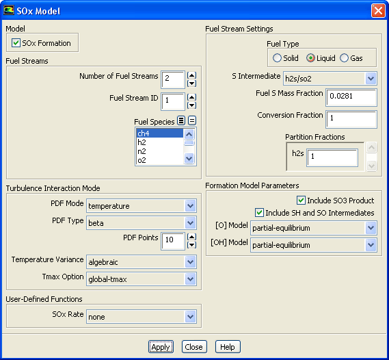
To model SOx formation, enable the SOx Formation option in the SOx Model dialog box (Figure  21.2.1).

Models SOx Edit...

Figure 21.2.1: The SOx Model Dialog Box

Defining the Fuel Streams

ANSYS FLUENT allows you to define multiple fuel streams when you are modeling SOx formation, as shown in the following steps:

1.   Specify the Number of Fuel Streams in the Fuel Streams group box. You are allowed up to three separate fuel streams.

2.   Define the first fuel stream.

(a)   Select the fuel stream to be defined by using the arrow keys of the Fuel Stream ID text box.

(b)   When the non-premixed combustion model is not enabled, select the fuel species from the Fuel Species list. You cannot select more than 5 fuel species for each fuel stream, and the total number of fuel species selected for all the fuel streams combined cannot exceed 10.

(c)   When the non-premixed combustion model is enabled (Figure  21.2.2), make a selection from the PDF Stream drop-down list to define the species for this stream. You can select either the primary or secondary fuel stream species, as defined in the PDF table.

(d)   Specify the parameters for this particular fuel stream in the Fuel Stream Settings group box. See Section  21.2.1 for details.

3.   Repeat steps 2.(a)-2.(c) for each additional fuel stream.

4.   Set the formation model parameters that apply to all of the fuel streams in the Formation Model Parameters group box:

• You have the option of including ${\rm SO}_3$ as a product, and including SH and SO as intermediates by enabling the Include SO3 Product and the Include SH and SO Intermediates options, respectively. See this section in the separate Theory Guide for further information.

• Specify the method by which O and OH will be calculated. The SOx routines employ three methods for reduction calculations of SOx:
  • You can select equilibrium, partial-equilibrium, or instantaneous in the [O] Model drop-down list.

  • You can select none, partial-equilibrium, or instantaneous in the [OH] Model drop-down list.

  To use the predicted O and/or OH concentration, select instantaneous in the [O] Model or [OH] Model drop-down list.

Figure 21.2.2: The SOx Model Dialog Box with Non-Premixed Combustion

Note that the following limitations apply when you are modeling SOx formation with multiple fuel streams, if more than one fuel stream has the same fuel type (as defined in the Fuel Type list in the Fuel Stream Settings group box):

• For multiple liquid fuel streams or multiple solid (coal) fuel streams, the injectors associated with the fuel streams should have different destination species, as defined in the Devolatilizing Species drop-down list in the Set Injection Properties dialog box (see Section  23.3.15 for details). The SOx calculations will be erroneous if the destination species are the same.

• For multiple solid (coal) fuel streams, the fuel streams should have the same char-related parameter values in the Fuel Stream Settings group box--i.e., the Char S Mass Fraction and the Partition Fractions (for char S) values. Note that even if different values are set for these char-related parameters, ANSYS FLUENT will only recognize those specified for the solid fuel stream with the lowest ID number, and then apply them to all of the other solid fuel streams.

For more information about the limitations associated with multiple fuel streams with the same fuel type, contact your ANSYS FLUENT support engineer.

Note that if you read a case file with SOx settings that was set up in a version of ANSYS FLUENT previous to 12, you must make a selection for the fuel species. This selection should be made either in the PDF Stream drop-down list for non-premixed combustion, or in the Fuel Species list for all other combustion models.

Defining the SOx Fuel Stream Settings

When using the SOx model, you must set the parameters in the Fuel Stream Settings group box for each fuel stream specified in the Fuel Stream ID text box.

To begin, specify the fuel type in the following manner:

• To calculate SOx formation from a solid fuel, select Solid under Fuel Type.

• To calculate SOx formation from a liquid fuel, select Liquid under Fuel Type.

• To calculate SOx formation from a gaseous fuel, select Gas under Fuel Type.

Figure 21.2.3: The SOx Model Dialog Box Displaying Liquid Fuel Parameters

Note that you can use only one of the fuel types for a given fuel stream. The Gas option is available only when the Species Transport model is enabled (see Section  15.1.2).

Setting SOx Parameters for Gaseous and Liquid Fuel Types

If you have selected Gas or Liquid as the Fuel Type, you will also need to specify the following:

• Select the intermediate species ( h2s, so2, or h2s/so2) in the S Intermediate drop-down list.

• Set the correct mass fraction of sulfur in the fuel (kg sulfur per kg fuel) in the Fuel S Mass Fraction field.

• Specify the overall fraction of the fuel S, by mass, that will be converted to the intermediate species and/or product SO $_2$ in the Conversion Fraction field. Thus, any remaining S will not contribute to SOx formation. This is based on the assumption that the remaining volatile S will convert to gas phase sulfur. The Conversion Fraction for the S Intermediate has a default value of 1.

• If you selected h2s/so2 as the intermediate, you will need to set the fraction of the converted fuel S, by mass, that will become h2s under Partition Fractions. The fraction of fuel S that will become SO $_2$ will be calculated by the remainder.

  Note that setting a partition fraction of 0 for H $_2$S is equivalent to assuming that all fuel S is converted to the final product SO $_2$.

Note that there is a limitation that must be considered when defining more than one liquid fuel stream. See Section  21.1.1 for details.

Setting SOx Parameters for a Solid Fuel

For solid fuel, several inputs are required for the SOx model.

Figure 21.2.4: The SOx Model Dialog Box Displaying Solid Fuel Parameters

• Select the intermediate species ( h2s, so2, or h2s/so2) in the S Intermediate drop-down list.

• Specify the mass fraction of sulfur in the volatiles in the Volatile S Mass Fraction field.

• Specify the overall fraction of the volatile S, by mass, that will be converted to the intermediate species and/or product SO $_2$ in the Conversion Fraction field.

• If you selected h2s/so2 as the volatile S intermediate, you will need to specify the fraction of the converted volatile S, by mass, that will become h2s under Partition Fractions. The fraction of volatile S that will become SO $_2$ will be calculated by the remainder.

• Select the char S conversion path from the Char S Conversion drop-down list as so2, h2s, or so2/h2s.

• Specify the mass fraction of sulfur in the char in the Char S Mass Fraction field.

• Specify the overall fraction of the char S, by mass, that will be converted to the intermediate species and/or product SO $_2$ in the Conversion Fraction field.

• If you selected so2/h2s from the Char S Conversion drop-down list, you will need to specify the fraction of the converted char S, by mass, that will become ${\rm SO}_2$ under Partition Fractions. The fraction of char S that will become H $_2$S will be calculated by the remainder.

Note that there are limitations that must be considered when defining more than one solid fuel stream. See Section  21.2.1 for details.

The following equations are used to determine the mass fraction of sulfur in the volatiles and char:

where
	$\dot{m}_{S_{v/c}}$	= rate of release of fuel sulfur in kg/s
	$\dot{m}_{v/c}$	= rate of release of volatiles (v) or char (c) in kg/s
	$mf_{S_{v/c}}$	= mass fraction of sulfur in volatiles or char

Let
	$TS_{fuel}$	= total sulfur mass fraction in daf coal (i.e., from daf ultimate analysis)
	$S_{split}$	= char sulfur as a fraction of total sulfur
	$F_{vol}$	= mass fraction of volatiles in daf coal
	$F_{char}$	= mass fraction of char in daf coal

Then the following should hold:

Note that if water is assumed to release at the same rate as volatiles, the above calculation has to be slightly modified.

Setting Turbulence Parameters

If you want to take into account turbulent fluctuations when you compute the specified SO $_2$ formation, define the turbulence parameters in the Turbulence Interaction Mode group box.

Figure 21.2.5: The SOx Model Dialog Box for a Gas Fuel Type with Turbulence

Select one of the options in the PDF Mode drop-down list:

• Select temperature to take into account fluctuations of temperature.

• Select temperature/species to take into account fluctuations of temperature and mass fraction of the species selected in the Species drop-down list (which appears when you select this option).

• (non-premixed and partially premixed combustion calculations only) Select mixture fraction to take into account fluctuation in the mixture fraction(s).

When modeling the formation of other pollutants along with SOx, you should compare the selections made in the PDF Mode drop-down lists in the Turbulence Interaction Mode tab of the NOx Model dialog box and the Turbulence Interaction Mode group boxes of the SOx Model and Soot Model dialog boxes. If mixture fraction is selected in any of these dialog boxes, then it must be selected in all of the others as well.

The mixture fraction option is available only if you are using either the non-premixed or partially premixed combustion model to model the reacting system. If you use the mixture fraction option, the instantaneous temperatures and species concentrations are taken from the PDF look-up table as a function of mixture fraction and enthalpy and the instantaneous SOx rates are calculated at each cell. The PDF used for convoluting the instantaneous SOx rates is the same as the one used to compute the mean flow-field properties. For example, for single-mixture fraction models the beta PDF is used, and for two-mixture fraction models, the beta or the double delta PDF can be used. The PDF for mixture fraction is calculated from the values of mean mixture fraction and variance at each cell, and the instantaneous SOx rates are convoluted with the mixture fraction PDF to yield the mean rates in turbulent flow.

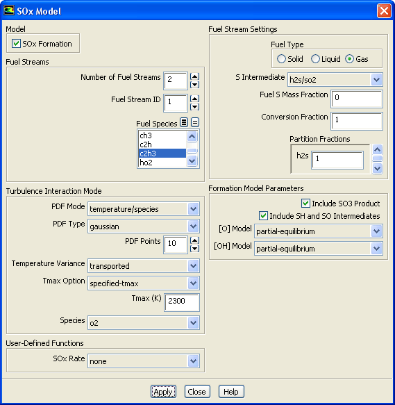
If you selected temperature or temperature/species for the PDF Mode, you should define the following parameters in the Turbulence Interaction Mode group box:

PDF Type   allows you to specify the shape of the PDF, which is then integrated to obtain mean rates for the temperature and (if you selected temperature/species for the PDF Mode) the species. If you select beta, the PDF will be modeled using this equation in the separate Theory Guide. If you select gaussian, the PDF will be modeled using this equation in the separate Theory Guide.

PDF Points   allows you to specify the number of points used to integrate the beta or Gaussian function in this equation or this equation in the separate Theory Guide on a histogram basis. The default value of 10 will yield an accurate solution with reasonable computation time. Increasing this value may improve accuracy, but will also increase the computation time.

Temperature Variance   allows you to specify the form of transport equation that is solved to calculate the temperature variance. The default selection is algebraic, which is an approximate form of the transport equation (see this equation in the separate Theory Guide). You have the option of selecting transported to instead solve this equation in the separate Theory Guide. Though the transported form is more exact, it is also more expensive computationally.

Tmax Option   provides various options for determining the maximum limit(s) for the integration of the PDF used to calculate the temperature:

• The default selection is global-tmax, which sets the limit as the maximum temperature in the flow field.

• You can select local-tmax if you would rather obtain cell-based maximum temperature limits by multiplying the local cell mean temperature by the value entered in Tmax Factor.

• You can select specified-tmax to set the limit for each cell to be the value entered in Tmax.

• If you have selected a user-defined function from the SOx Rate drop-down menu in the User-Defined Functions group box, then you can select user-defined so that the limit is specified by a UDF. See the separate UDF Manual for details about user-defined functions.

Species   only appears if you have selected temperature/species for the PDF Mode. Your selection in this drop-down menu determines which species' mass fraction is included in the SOx formation calculations.

Note that the species variance will always be calculated using the algebraic form of the transport equation ( this equation in the separate Theory Guide).

Specifying a User-Defined Function for the SOx Rate

You can choose to specify a user-defined function for the rate of SOx production. By default, the rate returned from the UDF is added to the rate returned from the standard SOx production options. You also have the option of replacing ANSYS FLUENT's SOx rate calculations with your own user-defined SOx rate.

In addition to or instead of using the UDF to specify the SOx rate, you can use it to specify custom values for the maximum limit ( $T_{\rm max}$) that is used for the integration of the temperature PDF (when temperature is accounted for in the turbulence interaction modeling).

To use a UDF to add a rate to ANSYS FLUENT's SOx rate calculations, you must compile and load the desired function, and then select it from the SOx Rate drop-down list in the User-Defined Functions group box. After you have selected the UDF, you have the following options:

• You can specify that your custom rate is added to the ANSYS FLUENT SOx rate calculations, by retaining the default selection of Add to the FLUENT Rate in the UDF Rate group box.

• You can replace the ANSYS FLUENT SOx rate calculations with your custom rate, by selecting Replace FLUENT Rate in the UDF Rate group box.

• You can specify custom values for $T_{\rm max}$, by selecting user-defined from the Tmax Option drop-down list in the Turbulence Interaction Mode group box.

See the separate UDF Manual for details about user-defined functions.

Defining Boundary Conditions for the SOx Model

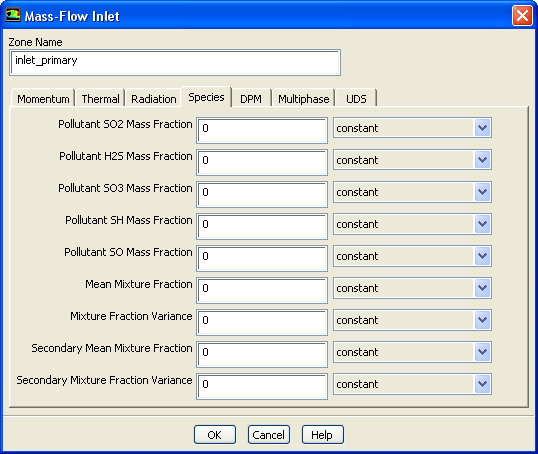
At flow inlet boundaries, you will need to specify the Pollutant SO Mass Fraction, and if necessary, the Pollutant SH Mass Fraction, Pollutant H2S Mass Fraction, Pollutant SO3 Mass Fraction,and Pollutant SO2 Mass Fraction in the Species tab, as demonstrated in Figure  21.2.6.

Boundary Conditions

You can retain the default inlet values of zero for these quantities or you can input nonzero numbers as appropriate for your combustion system.

Figure 21.2.6: The Mass-Flow Inlet Dialog Box and the Species Tab