![[ANSYS, Inc. Logo]](fluentlogo.gif)


|
|
|
The devolatilization law
is applied to a combusting particle when the temperature of the particle reaches the vaporization
temperature,
 , and remains in effect while the mass of the particle,
 , exceeds the mass of the nonvolatiles in the particle:
and
where
 is the mass fraction of the evaporating/boiling material if
Wet Combustion is selected (otherwise,
is the mass fraction of the evaporating/boiling material if
Wet Combustion is selected (otherwise,
 ). As implied by Equation
15.4-24, the boiling point,
). As implied by Equation
15.4-24, the boiling point,
 , and the vaporization temperature,
 , should be set equal to each other when Law 4 is to be used. When wet combustion is active,
 and
and
 refer to the boiling and evaporation temperatures for the combusting material only.
ANSYS FLUENT provides a choice of four devolatilization models:
Each of these models is described, in turn, below.
Choosing the Devolatilization Model
You will choose the devolatilization model when you are setting physical properties for the combusting-particle material in the Create/Edit Materials dialog box, as described in this section in the separate User's Guide. By default, the constant rate model (Equation 15.4-26) will be used.
The Constant Rate Devolatilization Model
The constant rate devolatilization law dictates that volatiles are released at a constant rate [ 20]:
| where |
 |
= | particle mass (kg) |
 |
= | fraction of volatiles initially present in the particle | |
 |
= | initial particle mass (kg) | |
 |
= | rate constant (s
 ) ) |
The rate constant
 is defined as part of your modeling inputs, with a default value of 12 s
 derived from the work of Pillai [
271] on coal combustion. Proper use of the constant devolatilization rate requires that the vaporization temperature, which controls the onset of devolatilization, be set appropriately. Values in the literature show this temperature to be about 600 K [
20].
derived from the work of Pillai [
271] on coal combustion. Proper use of the constant devolatilization rate requires that the vaporization temperature, which controls the onset of devolatilization, be set appropriately. Values in the literature show this temperature to be about 600 K [
20].
The volatile fraction of the particle enters the gas phase as the devolatilizing species
 , defined by you (see
this section in the separate
User's Guide). Once in the gas phase, the volatiles may react according to the inputs governing the gas phase chemistry.
, defined by you (see
this section in the separate
User's Guide). Once in the gas phase, the volatiles may react according to the inputs governing the gas phase chemistry.
The Single Kinetic Rate Model
The single kinetic rate devolatilization model assumes that the rate of devolatilization is first-order dependent on the amount of volatiles remaining in the particle [ 10]:
| where |
 |
= | particle mass (kg) |
 |
= | mass fraction of volatiles initially present in the particle | |
 |
= | mass fraction of evaporating/boiling material (if wet combustion | |
| is modeled) | |||
 |
= | initial particle mass (kg) | |
 |
= | kinetic rate (s
 ) ) |
Note that
 , the fraction of volatiles in the particle, should be defined using a value slightly in excess of that determined by proximate analysis. The kinetic rate,
 , is defined by input of an Arrhenius type pre-exponential factor and an activation energy:
ANSYS FLUENT uses default rate constants,
 and
and
 [
10].
[
10].
Equation 15.4-27 has the approximate analytical solution:
which is obtained by assuming that the particle temperature varies only slightly between discrete time integration steps.
ANSYS FLUENT can also solve Equation 15.4-29 in conjunction with the equivalent heat transfer equation using a stiff coupled solver. See this section in the separate User's Guide for details.
The Two Competing Rates (Kobayashi) Model
ANSYS FLUENT also provides the kinetic devolatilization rate expressions of the form proposed by Kobayashi [ 169]:
where
 and
and
 are competing rates that may control the devolatilization over different temperature ranges. The two kinetic rates are weighted to yield an expression for the devolatilization as
| where |
 |
= | volatile yield up to time
 |
 |
= | initial particle mass at injection | |
 |
= | yield factors | |
 |
= | ash content in the particle |
The Kobayashi model requires input of the kinetic rate parameters,
 ,
,
 ,
,
 , and
, and
 , and the yields of the two competing reactions,
 and
and
 .
ANSYS FLUENT uses default values for the yield factors of 0.3 for the first (slow) reaction and 1.0 for the second (fast) reaction. It is recommended in the literature [
169] that
.
ANSYS FLUENT uses default values for the yield factors of 0.3 for the first (slow) reaction and 1.0 for the second (fast) reaction. It is recommended in the literature [
169] that
 be set to the fraction of volatiles determined by proximate analysis, since this rate represents devolatilization at low temperature. The second yield parameter,
 , should be set close to unity, which is the yield of volatiles at very high temperature.
By default, Equation 15.4-32 is integrated in time analytically, assuming the particle temperature to be constant over the discrete time integration step. ANSYS FLUENT can also solve Equation 15.4-32 in conjunction with the equivalent heat transfer equation using a stiff coupled solver. See this section in the separate User's Guide for details.
The CPD Model
In contrast to the coal devolatilization models presented above, which are based on empirical rate relationships, the chemical percolation devolatilization (CPD) model characterizes the devolatilization behavior of rapidly heated coal based on the physical and chemical transformations of the coal structure [ 100, 101, 116].
General Description
During coal pyrolysis, the labile bonds between the aromatic clusters in the coal structure lattice are cleaved, resulting in two general classes of fragments. One set of fragments has a low molecular weight (and correspondingly high vapor pressure) and escapes from the coal particle as a light gas. The other set of fragments consists of tar gas precursors that have a relatively high molecular weight (and correspondingly low vapor pressure) and tend to remain in the coal for a long period of time during typical devolatilization conditions. During this time, reattachment with the coal lattice (which is referred to as crosslinking) can occur. The high molecular weight compounds plus the residual lattice are referred to as metaplast. The softening behavior of a coal particle is determined by the quantity and nature of the metaplast generated during devolatilization. The portion of the lattice structure that remains after devolatilization is comprised of char and mineral-compound-based ash.
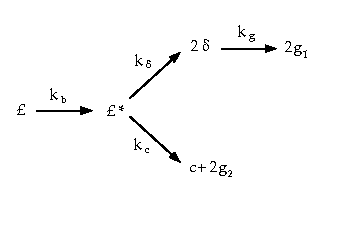
The CPD model characterizes the chemical and physical processes by considering the coal structure as a simplified lattice or network of chemical bridges that link the aromatic clusters. Modeling the cleavage of the bridges and the generation of light gas, char, and tar precursors is then considered to be analogous to the chemical reaction scheme shown in Figure 15.4.1.
The variable
 represents the original population of labile bridges in the coal lattice. Upon heating, these bridges become the set of reactive bridges,
 . For the reactive bridges, two competing paths are available. In one path, the bridges react to form side chains,
 . The side chains may detach from the aromatic clusters to form light gas,
 . As bridges between neighboring aromatic clusters are cleaved, a certain fraction of the coal becomes detached from the coal lattice. These detached aromatic clusters are the heavy-molecular-weight tar precursors that form the metaplast. The metaplast vaporizes to form coal tar. While waiting for vaporization, the metaplast can also reattach to the coal lattice matrix (crosslinking). In the other path, the bridges react and become a char bridge,
 , with the release of an associated light gas product,
 . The total population of bridges in the coal lattice matrix can be represented by the variable
 , where
 .
.
Reaction Rates
Given this set of variables that characterizes the coal lattice structure during devolatilization, the following set of reaction rate expressions can be defined for each, starting with the assumption that the reactive bridges are destroyed at the same rate at which they are created (
 ):
):
where the rate constants for bridge breaking and gas release steps,
 and
and
 , are expressed in Arrhenius form with a distributed activation energy:
where
 ,
,
 , and
, and
 are, respectively, the pre-exponential factor, the activation energy, and the distributed variation in the activation energy,
 is the universal gas constant, and
 is the temperature. The ratio of rate constants,
 , is set to 0.9 in this model based on experimental data.
Mass Conservation
The following mass conservation relationships are imposed:
where
 is the fraction of broken bridges (
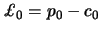
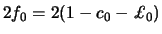
 ). The initial conditions for this system are given by the following:
where
 is the initial fraction of char bridges,
 is the initial fraction of bridges in the coal lattice, and
 is the initial fraction of labile bridges in the coal lattice.
Fractional Change in the Coal Mass
Given the set of reaction equations for the coal structure parameters, it is necessary to relate these quantities to changes in coal mass and the related release of volatile products. To accomplish this, the fractional change in the coal mass as a function of time is divided into three parts: light gas (
 ), tar precursor fragments (
 ), and char (
 ). This is accomplished by using the following relationships, which are obtained using percolation lattice statistics:
The variables
 ,
,
 ,
,
 , and
, and
 are the statistical relationships related to the cleaving of bridges based on the percolation lattice statistics, and are given by the following equations:
 is the ratio of bridge mass to site mass,
 , where
where
 and
and
 are the side chain and cluster molecular weights respectively.
 is the lattice coordination number, which is determined from solid-state nuclear magnetic Resonance (NMR) measurements related to coal structure parameters, and
 is the root of the following equation in
 (the total number of bridges in the coal lattice matrix):
In accounting for mass in the metaplast (tar precursor fragments), the part that vaporizes is treated in a manner similar to flash vaporization, where it is assumed that the finite fragments undergo vapor/liquid phase equilibration on a time scale that is rapid with respect to the bridge reactions. As an estimate of the vapor/liquid that is present at any time, a vapor pressure correlation based on a simple form of Raoult's Law is used. The vapor pressure treatment is largely responsible for predicting pressure-dependent devolatilization yields. For the part of the metaplast that reattaches to the coal lattice, a cross-linking rate expression given by the following equation is used:
where
 is the amount of mass reattaching to the matrix,
 is the amount of mass in the tar precursor fragments (metaplast), and
 and
and
 are rate expression constants.
CPD Inputs
Given the set of equations and corresponding rate constants introduced for the CPD model, the number of constants that must be defined to use the model is a primary concern. For the relationships defined previously, it can be shown that the following parameters are coal independent [ 100]:
 ,
,
 ,
,
 ,
,
 ,
,
 , and
, and
 for the rate constants
 and
and

 ,
,
 , and
, and

These constants are included in the submodel formulation and are not input or modified during problem setup.
There are an additional five parameters that are coal-specific and must be specified during the problem setup:


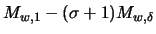
The first four of these are coal structure quantities that are obtained from NMR experimental data. The last quantity, representing the char bridges that either exist in the parent coal or are formed very early in the devolatilization process, is estimated based on the coal rank. These quantities are entered in the Create/Edit Materials dialog box, as described in this section in the separate User's Guide. Values for the coal-dependent parameters for a variety of coals are listed in Table 15.4.1.
| Coal Type |
 |
 |
 |
 |
 |
| Zap (AR) | 3.9 | .63 | 277 | 40 | .20 |
| Wyodak (AR) | 5.6 | .55 | 410 | 42 | .14 |
| Utah (AR) | 5.1 | .49 | 359 | 36 | 0 |
| Ill6 (AR) | 5.0 | .63 | 316 | 27 | 0 |
| Pitt8 (AR) | 4.5 | .62 | 294 | 24 | 0 |
| Stockton (AR) | 4.8 | .69 | 275 | 20 | 0 |
| Freeport (AR) | 5.3 | .67 | 302 | 17 | 0 |
| Pocahontas (AR) | 4.4 | .74 | 299 | 14 | .20 |
| Blue (Sandia) | 5.0 | .42 | 410 | 47 | .15 |
| Rose (AFR) | 5.8 | .57 | 459 | 48 | .10 |
| 1443 (lignite, ACERC) | 4.8 | .59 | 297 | 36 | .20 |
| 1488 (subbituminous, ACERC) | 4.7 | .54 | 310 | 37 | .15 |
| 1468 (anthracite, ACERC) | 4.7 | .89 | 656 | 12 | .25 |
Particle Swelling During Devolatilization
The particle diameter changes during devolatilization according to the swelling coefficient,
 , which is defined by you and applied in the following relationship:
| where |
 |
= | particle diameter at the start of devolatilization |
 |
= | current particle diameter |
The term
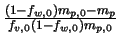 is the ratio of the mass that has been devolatilized to the total volatile mass of the particle. This quantity approaches a value of 1.0 as the devolatilization law is applied. When the swelling coefficient is equal to 1.0, the particle diameter stays constant. When the swelling coefficient is equal to 2.0, the final particle diameter doubles when all of the volatile component has vaporized, and when the swelling coefficient is equal to 0.5 the final particle diameter is half of its initial diameter.
Heat Transfer to the Particle During Devolatilization
Heat transfer to the particle during the devolatilization process includes contributions from convection, radiation (if active), and the heat consumed during devolatilization:
Radiation heat transfer to the particle is included only if you have enabled the P-1 or discrete ordinates radiation model and you have activated radiation heat transfer to particles using the Particle Radiation Interaction option in the Discrete Phase Model dialog box.
By default, Equation 15.4-58 is solved analytically, by assuming that the temperature and mass of the particle do not change significantly between time steps:
![T_p (t + \Delta t) = \alpha_p + [T_p (t) - \alpha_p] e^{-\beta_p \Delta t}](img6188.gif) |
(15.4-59) |
where
 |
(15.4-60) |
and
 |
(15.4-61) |
ANSYS FLUENT can also solve Equation 15.4-58 in conjunction with the equivalent mass transfer equation using a stiff coupled solver. See this section in the separate User's Guide for details.
Previous:
15.4.3 Droplet Boiling (Law



![- \frac{d m_p}{dt} = k [ m_p - (1 - f_{v,0})(1 - f_{w,0}) m_{p,0} ]](img6021.gif)

![m_p (t + \Delta t) = (1 - f_{v,0})(1- f_{w,0})m_{p,0} + [ m_p (t) - (1 -f_{v,0})(1 - f_{w,0} )m_{p,0} ] e^{-k \Delta t}](img6033.gif)





![$\displaystyle \left[ 2 \rho k_b \frac{\pounds}{\rho + 1} \right] -k_g \delta$](img6070.gif)









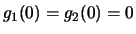


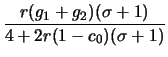


![$\displaystyle \frac{2}{2+r(1-c_0)(\sigma+1)} \left[\Phi F(p) + r \Omega K(p) \right]$](img6120.gif)


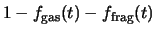


![$\displaystyle 1+r \left[\frac{\pounds}{p} + \frac{(\sigma-1) \delta}{4(1 - p)} \right]$](img6130.gif)


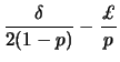


![$\displaystyle \left[ 1 - \left(\frac{\sigma+1}{2} \right) p' \right] \left(\frac{p'}{p} \right) ^{\frac{\sigma+1}{\sigma-1}}$](img6139.gif)




 C NMR for 13 Coals
