![[ANSYS, Inc. Logo]](fluentlogo.gif)


|
|
|
The Lagrangian solution method solves the composition PDF transport equation by stochastically tracking Lagrangian particles through the domain. It is computationally expensive since a large number of particles are required to represent the PDF, and a large number of iterations are necessary to reduce statistical errors and explicitly convect the particles through the domain. The Eulerian PDF transport model overcomes these limitations by assuming a shape for the PDF, which allows Eulerian transport equations to be derived. Stochastic errors are eliminated and the transport equations are solved implicitly, which is computationally economical. The multi-dimensional PDF shape is assumed as a product of delta functions. As with the Lagrangian PDF model, the highly non-linear chemical source term is closed. However, the turbulent scalar flux and molecular mixing terms must be modeled, and are closed with the gradient diffusion and the IEM models, respectively.
The composition PDF of
 dimension (
 species and enthalpy) is represented as a collection of
 delta functions (or modes). This presumed PDF has the following form:
where
 is the probability in each mode,
 is the conditional mean composition of specie
 in the
 th mode,
 is the composition space variable of specie
 , and
, and
 is the delta function.
The Eulerian PDF transport equations are derived by substituting Equation
11.4-1 into the closed composition PDF transport equation (Equation
11.2-1 with Equations
11.2-2 and
11.3-6). The unknown terms,
 and
and
 , are determined by forcing lower moments of this transported PDF to match the RANS lower moment transport equations, using the Direct Quadrature Method of Moments (DQMOM) approach [
103,
218]. The resulting transport equations are:
, are determined by forcing lower moments of this transported PDF to match the RANS lower moment transport equations, using the Direct Quadrature Method of Moments (DQMOM) approach [
103,
218]. The resulting transport equations are:
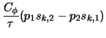
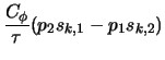
 th delta function):
 :
:
where
 is the probability of the
 th mode, and
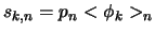 is the
 th specie probability weighted conditional mean composition of the
 th mode.
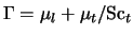 is the effective turbulent diffusivity. The terms
 ,
,
 and
and
 represent mixing, reaction and correction terms respectively. Note that only
 probability equations are solved and the
 th probability is calculated as one minus the sum of the
 solved probabilities.
Reaction
The reaction source term
 in Equation
11.4-3 for the
in Equation
11.4-3 for the
 th composition and the
 th mode is calculated as,
 |
(11.4-4) |
where
 is the net reaction rate for the
 th component.
Mixing
The micro-mixing term
 is modeled with the IEM mixing model:
 |
(11.4-5) |
where
 is the turbulence time-scale and
 is the mixing constant.
Hence, for the two-mode DQMOM-IEM model, the mixing terms for component
 are,
are,
The default value of
 is 2, which is appropriate for gas-phase combustion. For reactions in liquids, where the diffusivities are much smaller than gases, the
Liquid Micro-Mixing option interpolates
is 2, which is appropriate for gas-phase combustion. For reactions in liquids, where the diffusivities are much smaller than gases, the
Liquid Micro-Mixing option interpolates
 from model turbulence [
278] and scalar [
103] spectra.
from model turbulence [
278] and scalar [
103] spectra.
Correction
Using assumptions to ensure realizability and boundedness, the correction terms
 in Equation
11.4-3 for the
in Equation
11.4-3 for the
 th composition are determined from the linear system,
where
 are the non-negative integer lower moments (1..
 ) for each component
 . Note that the condition of the matrix decreases with increasing
 , which reduces the stability of higher mode simulations.
The dissipation term
 in Equation
11.4-7 is calculated as,
in Equation
11.4-7 is calculated as,
 |
(11.4-8) |
For the two-mode DQMOM-IEM model, the correction terms for the
 th component are,
Calculation of Composition Mean and Variance
The mean composition (specie
 or energy) is calculated as,
 |
(11.4-10) |
and its variance is calculated as
 |
(11.4-11) |
Previous:
11.3.4 The ISAT Algorithm
![P(\psi;\vec{x},t) = \sum_{n=1}^{N_e} p_n(\vec{x},t) \prod_{k=1}^{N_s} \delta[\psi_k - <\phi_k>_n (\vec{x},t)]](img4211.gif)