8.4.2 The Flamelet Concept

Overview

The flamelet concept views the turbulent flame as an ensemble of thin, laminar, locally one-dimensional flamelet structures embedded within the turbulent flow field [ 36, 267, 268] (see Figure  8.4.1).

Figure 8.4.1: Laminar Opposed-Flow Diffusion Flamelet

A common laminar flame type used to represent a flamelet in a turbulent flow is the counterflow diffusion flame. This geometry consists of opposed, axisymmetric fuel and oxidizer jets. As the distance between the jets is decreased and/or the velocity of the jets increased, the flame is strained and increasingly departs from chemical equilibrium until it is eventually extinguished. The species mass fraction and temperature fields can be measured in laminar counterflow diffusion flame experiments, or, most commonly, calculated. For the latter, a self-similar solution exists, and the governing equations can be simplified to one dimension along the axis of the fuel and oxidizer jets, where complex chemistry calculations can be affordably performed.

In the laminar counterflow flame, the mixture fraction, $f$, (see Section  8.2.1 for definition) decreases monotonically from unity at the fuel jet to zero at the oxidizer jet. If the species mass fraction and temperature along the axis are mapped from physical space to mixture fraction space, they can be uniquely described by two parameters: the mixture fraction and the strain rate (or, equivalently, the scalar dissipation, $\chi$, defined in Equation  8.4-2). Hence, the chemistry is reduced and completely described by the two quantities, $f$ and $\chi$.

This reduction of the complex chemistry to two variables allows the flamelet calculations to be preprocessed, and stored in look-up tables. By preprocessing the chemistry, computational costs are reduced considerably.

The balance equations, solution methods, and sample calculations of the counterflow laminar diffusion flame can be found in several references. Comprehensive reviews and analyses are presented in the works of Bray and Peters, and Dixon-Lewis [ 36, 72].

Strain Rate and Scalar Dissipation

A characteristic strain rate for a counterflow diffusion flamelet can be defined as $a_s = v/2d$, where $v$ is the relative speed of the fuel and oxidizer jets, and $d$ is the distance between the jet nozzles.

Instead of using the strain rate to quantify the departure from equilibrium, it is expedient to use the scalar dissipation, denoted by $\chi$. The scalar dissipation is defined as

where $D$ is a representative diffusion coefficient.

Note that the scalar dissipation, $\chi$, varies along the axis of the flamelet. For the counterflow geometry, the flamelet strain rate $a_s$ can be related to the scalar dissipation at the position where $f$ is stoichiometric by [ 267]:

where
	$\chi_{\rm st}$	= scalar dissipation at $f=f_{\rm st}$
	$a_s$	= characteristic strain rate
	$f_{\rm st}$	= stoichiometric mixture fraction
	${\rm erfc}^{-1}$	= inverse complementary error function

Physically, as the flame is strained, the width of the reaction zone diminishes, and the gradient of $f$ at the stoichiometric position $f=f_{\rm st}$ increases. The instantaneous stoichiometric scalar dissipation, $\chi_{\rm st}$, is used as the essential non-equilibrium parameter. It has the dimensions s $^{-1}$ and may be interpreted as the inverse of a characteristic diffusion time. In the limit $\chi_{\rm st} \rightarrow 0$ the chemistry tends to equilibrium, and as $\chi_{\rm st}$ increases due to aerodynamic straining, the non-equilibrium increases. Local quenching of the flamelet occurs when $\chi_{\rm st}$ exceeds a critical value.

Embedding Laminar Flamelets in Turbulent Flames

A turbulent flame brush is modeled as an ensemble of discrete laminar flamelets. Since, for adiabatic systems, the species mass fraction and temperature in the laminar flamelets are completely parameterized by $f$ and $\chi_{\rm st}$, density-weighted mean species mass fractions and temperature in the turbulent flame can be determined from the PDF of $f$ and $\chi_{\rm st}$ as

where $\phi$ represents species mass fractions and temperature.

In ANSYS FLUENT, $f$ and $\chi_{\rm st}$ are assumed to be statistically independent, so the joint PDF $p(f,\chi_{\rm st})$ can be simplified as 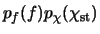$p_{f}(f)p_{\chi}(\chi_{\rm st})$. A $\beta$ PDF shape is assumed for $p_f$, and transport equations for $\overline{f}$ and $\overline{f^{'2}}$ are solved in ANSYS FLUENT to specify $p_f$. Fluctuations in $\chi_{\rm st}$ are ignored so that the PDF of $\chi$ is a delta function: 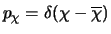$p_{\chi} = \delta (\chi-\overline{\chi})$. The first moment, namely the mean scalar dissipation, $\overline{\chi_{\rm st}}$, is modeled in ANSYS FLUENT as

where $C_{\chi}$ is a constant with a default value of 2.

For LES, the mean scalar dissipation is modeled as

To avoid the PDF convolutions at ANSYS FLUENT run-time, the integrations in Equation  8.4-3 are preprocessed and stored in look-up tables. For adiabatic flows, flamelet tables have three dimensions: $\overline{f}$, $\overline{f^{'2}}$ and $\overline{\chi_{\rm st}}$.

For non-adiabatic steady laminar flamelets, the additional parameter of enthalpy is required. However, the computational cost of modeling steady flamelets over a range of enthalpies is prohibitive, so some approximations are made. Heat gain/loss to the system is assumed to have a negligible effect on the species mass fractions, and adiabatic mass fractions are used [ 27, 240]. The temperature is then calculated from Equation  5.2-7 for a range of mean enthalpy gain/loss, $\overline{H}$. Accordingly, mean temperature and density PDF tables have an extra dimension of mean enthalpy. The approximation of constant adiabatic species mass fractions is, however, not applied for the case corresponding to a scalar dissipation of zero. Such a case is represented by the non-adiabatic equilibrium solution. For $\overline{\chi_{\rm st}}=0$, the species mass fractions are computed as functions of $\overline{f}$, $\overline{f^{'2}}$, and $\overline{H}$.

In ANSYS FLUENT, you can either generate your own flamelets, or import them as flamelet files calculated with other stand-alone packages. Such stand-alone codes include OPPDIF [ 210] , CFX-RIF [ 15, 16, 272] and RUN-1DL [ 270]. ANSYS FLUENT can import flamelet files in OPPDIF format or standard flamelet file format.

Instructions for generating and importing flamelets are provided in Section  8.4.3 and Section  8.4.4.