29.9.4 XY Plots of Profiles

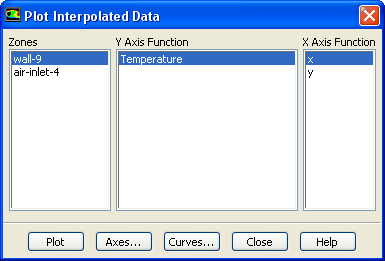
ANSYS FLUENT allows two options for generating XY plots of data related to boundary profiles. Using the Plot Profile Data dialog box, you can plot the original data points from the profile file you have read into ANSYS FLUENT. Alternatively, you can plot the values assigned to the cell faces on the boundary after the profile file has been interpolated, by using the Plot Interpolated Data dialog box.

Note that you must have valid data when trying to use the profile plotting options.

For more information about boundary profiles, see Section  7.6.

Steps for Generating Plots of Profile Data

Once you have read a profile file, it is available for plotting by using the Plot Profile Data dialog box.

Plots Profile Data Set Up...

Figure 29.9.8: The Plot Profile Data Dialog Box

The steps for generating a XY plot of the original profile data are as follows:

1.   Select one of the profiles you have read from the Profile selection list.

2.   Select a field of the profile from the Y Axis Function selection list.

3.   Choose a variable against which you want to plot the field data, and select it from the X Axis Function selection list. The available variables will vary depending on the profile, and include x, y, z, r, and time.

4.   Modify the attributes of the axes or curves as described in Sections  29.9.9 and 29.9.10.

5.   Click the Plot button to generate an XY plot of the profile field data.

Steps for Generating Plots of Interpolated Profile Data

To interpolate a profile you must first read a profile file for the case, and select a profile field in a boundary conditions dialog box (e.g., the Velocity Inlet dialog box). After the flow solution has been initialized, the cell face values of the boundary zone can be plotted by using the Plot Interpolated Data dialog box.

Plots Interpolated Data Set Up...

Figure 29.9.9: The Plot Interpolated Data Dialog Box

The steps for generating an XY plot of the interpolated data are as follows:

1.   Select a zone from the Zones selection list. Only the zones for which you have set a profile field as one or more of the parameters will be available in this list.

2.   Select a profile-related parameter of the zone from the Y Axis Function selection list. The name of the parameter will be the same as that of the drop-down list in the boundary condition dialog box from which the profile field was selected.

3.   Choose a variable against which you want to plot the field data, and select it from the X Axis Function selection list. The available variables are x, y, and (for 3D cases) z.

4.   Modify the attributes of the axes or curves as described in Sections  29.9.9 and 29.9.10.

5.   Click the Plot button to generate an XY plot of the cell face values on the boundary.