11.3.5 Steady-State Dynamic Mesh Applications

You can use dynamic meshes for steady-state applications as well as for transient applications. Some examples include: checking the valve application after reaching a steady-state valve position; or after a fluid-structure interface application has reached a steady-state solution.

There are no differences in the meshing aspect between steady-state cases and transient cases. Furthermore, setting up a steady-state simulation is similar to setting up a transient case, described in Section  11.3. However, there are a few differences which you should note:

• A CG_MOTION UDF is needed to specify the motion of the boundary: a transient profile used in transient cases cannot be used in steady-state cases.

• The dtime passed to the CG_MOTION UDF is 1 by default: if a displacement of 1mm is needed to move the boundary, you can specify the velocity to be 1e-3m/s.

• Dynamic mesh parameters can be different since an interpolation error is no longer a concern.

• If you have enabled local remeshing for your steady-state application, you can instruct ANSYS FLUENT to perform additional remeshing after the boundary has moved. This additional remeshing is based on skewness criteria, and can further increase the quality of your mesh. See Section  11.3.2 for further details.

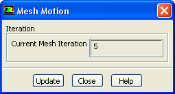
The mesh must be manually updated through journal files or execute commands. To update the mesh, you can use the Mesh Motion dialog box.

Run Calculation Preview Mesh Motion...

Alternatively, you can use the following text command:

solve $\rightarrow$ mesh-motion

which can also be used as an execute command in the Execute Commands dialog box:

Calculation Activities Create/Edit... (Execute Commands)

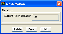
You can display dynamic mesh statistics (such as minimum and maximum volumes and maximum cell and face skewness) by clicking the Update button in the Mesh Motion dialog box (Figure  11.3.12).

Figure 11.3.12: The Mesh Motion Dialog Box for Steady-State Dynamic Meshes

The following options are not available for steady-state applications: In-Cylinder Six DOF Solver

An Example of Steady-State Dynamic Mesh Usage

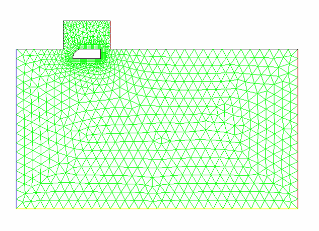
Consider a rescue drop case shown in Figure  11.3.13. The object can be moved in any position in the steady-state solver, after which steady-state analyses can be performed at different object positions.

Figure 11.3.13: Initial Object Position

The dynamic mesh parameters setup is identical for the steady-state and transient cases, which is described in Section  11.3.1. When setting up the dynamic zones, the procedures are similar to those described in Section  11.3.9, except that the UDF selected from the Motion UDF/Profile drop-down list is different. In steady-state cases the dtime passed to the UDF is by default 1. So, in this example, the object will move 50mm each time the following UDF is executed:

#include "udf.h"

DEFINE_CG_MOTION(pod,dt,vel,omega,time,dtime)

{
  NV_S(vel,=,0);
  NV_S(omega,=,0);

  vel[1] = -50e-3;
}

The resulting mesh is shown in Figure  11.3.15.

Figure 11.3.14: The Mesh Motion Dialog Box After 40 Updates

Figure 11.3.15: Final Object Position After 40 Executions