8.6.2 Anisotropic Diffusion

You can specify anisotropic diffusion coefficients in both fluid and solid zones by defining the tensor diffusion coefficient matrix $\Gamma$ (Equation  8.6-1) on a per-scalar basis. You can use anisotropic diffusivity for UDS scalar transport equations to model species transport equations in porous media and in solids where species diffusion shows anisotropic behavior.

Note that the anisotropic diffusion options discussed in the following sections are available with the pressure-based solver and the density-based solvers.

UDS diffusion coefficients can be postprocessed only in those cells which have isotropic diffusivity. In all other cells, the diffusion coefficient will be zero.

In all cases, you enable anisotropic diffusion by selecting defined-per-uds under UDS Diffusivity in the Create/Edit Materials dialog box. This will open the UDS Diffusion Coefficients dialog box (Figure  8.6.1).

Materials

In the UDS Diffusion Coefficient dialog box, select a scalar equation (e.g., uds-0) and then choose one of the following methods under Coefficient to specify the anisotropic diffusion coefficient. These methods are described in detail below.

• anisotropic

• orthotropic

• cylindrical orthotropic

• user-defined anisotropic

Anisotropic Diffusivity

For anisotropic diffusivity, you can specify $\Gamma$ in Equation  8.6-1 in the form $K\Gamma$ where $K$ is a constant $3x3$ matrix in 3D and $\Gamma$ is a scalar multiplier.

The diffusion coefficient matrix is specified as

where $k$ is the diffusivity and $\hat{\bf e}_{ij}$ is a matrix (2 $\times$ 2 for two dimensions and 3 $\times$ 3 for three-dimensional problems). Note that $\hat{\bf e}_{ij}$ can be a non-symmetric matrix.

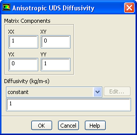
To specify anisotropic diffusion coefficients, first select a scalar equation (e.g., uds-0) from the User-Defined Scalar Diffusion list in the UDS Diffusion Coefficients dialog box (Figure  8.6.1). Then choose anisotropic in the drop-down list under Coefficient. This will open the Anisotropic UDS Diffusivity dialog box (Figure  8.6.2).

Figure 8.6.2: The Anisotropic UDS Diffusivity Dialog Box

In the Anisotropic UDS Diffusivity dialog box, enter the Matrix Components and then select the Diffusivity to be a constant, polynomial function of temperature ( polynomial, piecewise-linear, piecewise-polynomial), or user-defined. See Sections  8.2.1, 8.2.2, and 8.2.3 for details on polynomial temperature functions.

When you select the user-defined option, the User-Defined Functions dialog box will open allowing you to hook a DEFINE_DIFFUSIVITY UDF only if you have previously loaded a compiled UDF library or interpreted a UDF. Otherwise, you will get an error message. More information about user-defined functions can be found in the separate UDF Manual.

Orthotropic Diffusivity

For orthotropic diffusivity, you can specify $\Gamma$ in Equation  8.6-1 through 'principal' direction vectors and diffusion coefficients along these directions. ANSYS FLUENT, in turn, computes $\Gamma$ from parameters that you supply. The principal directions are the same everywhere, but each of he directional diffusion coefficients can be specified as a constant, polynomial function of temperature, or through user-defined functions.

When orthotropic diffusivity is used, the diffusion coefficients $(k_\xi,k_\eta,k_\zeta)$ in the principal directions $(\hat{\bf e}_\xi,\hat{\bf e}_\eta,\hat{\bf e}_\zeta)$ are specified. The diffusivity matrix is then computed as

For two-dimensional problems, only the functions $(k_\xi,k_\eta)$ and the unit vector $(\hat{\bf e}_\xi)$ need to be specified.

To specify orthotropic diffusion coefficients, first select a scalar equation (e.g., uds-0) from the User-Defined Scalar Diffusion list in the UDS Diffusion Coefficients dialog box (Figure  8.6.1). Then choose orthotropic in the drop-down list under Coefficient. This will open the Orthotropic UDS Diffusivity dialog box (Figure  8.6.3).

Figure 8.6.3: The Orthotropic UDS Diffusivity Dialog Box

Since the directions $(\hat{\bf e}_\xi,\hat{\bf e}_\eta,\hat{\bf e}_\zeta)$ are mutually orthogonal, only the first two need to be specified for three-dimensional problems. $\hat{\bf e}_\xi$ is defined using X,Y,Z under Direction 0 Components, and $\hat{\bf e}_\eta$ is defined using X,Y,Z under Direction 1 Components. You can define Diffusivity 0 $(k_\xi)$, Diffusivity 1 $(k_\eta)$, and Diffusivity 2 $(k_\zeta)$ as constant, polynomial, piecewise-linear, piecewise-polynomial functions of temperature, or user-defined. See Sections  8.2.1, 8.2.2, and 8.2.3 for details on polynomial temperature functions.

When you select the user-defined option, the User-Defined Functions dialog box will open allowing you to hook a DEFINE_DIFFUSIVITY UDF only if you have previously loaded a compiled UDF library or interpreted a UDF. If no functions have been loaded, you will get an error message. More information about user-defined functions can be found in the separate UDF Manual.

Cylindrical Orthotropic Diffusivity

Orthotropic UDS diffusivity can also be specified on a per-scalar basis in cylindrical coordinates. This method is similar to orthotropic UDS diffusivity, except that the principal directions are specified as radial, tangential, and axial.

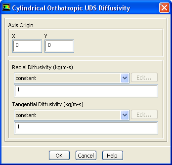
To specify cylindrical orthotropic diffusion coefficients, first select a scalar equation (e.g., uds-0) from the User-Defined Scalar Diffusion list in the UDS Diffusion Coefficients dialog box (Figure  8.6.1). Then choose cyl-orthotropic in the drop-down list under Coefficient. This will open the Cylindrical Orthotropic UDS Diffusivity dialog box (Figure  8.6.4).

Figure 8.6.4: The Cylindrical Orthotropic UDS Diffusivity Dialog Box

In three-dimensional cases, the origin and the direction of the cylindrical coordinate system must be specified along with the radial, tangential, and axial direction conductivities. In two-dimensional cases, the origin of the cylindrical coordinate system must be specified along with the radial and tangential direction conductivities. Note that in two-dimensional cases, the direction is always along the + z axis. ANSYS FLUENT will automatically compute the anisotropic diffusivity matrix at each cell from this input. The calculation is based on the location of the cell in the cylindrical coordinate system specified.

You can define the Radial Diffusivity, Tangential Diffusivity, and Axial Diffusivity as constant, polynomial, piecewise-linear, piecewise-polynomial, or as user-defined functions of temperature, using the drop-down list below each of the diffusivities. See Sections  8.2.1, 8.2.2, and 8.2.3 for details on polynomial temperature functions.

When you select the user-defined option, the User-Defined Functions dialog box will open allowing you to hook a DEFINE_DIFFUSIVITY UDF only if you have previously loaded a compiled UDF library or interpreted a UDF. If no functions have been loaded, you will get an error message. More information about user-defined functions can be found in the separate UDF Manual.