4.10.2 Realizable $k$- $\epsilon$ Based DES Model

This DES model is similar to the Realizable $k$- $\epsilon$ model discussed in Section  4.4.3, with the exception of the dissipation term in the $k$ equation. In the DES model, the Realizable $k$- $\epsilon$ RANS dissipation term is modified such that:

where

$$l_{des} = min (l_{rke}, l_{les})$$ (4.10-5)

$$l_{rke} = \frac{k^{\frac{3}{2}}}{\epsilon}$$ (4.10-6)

$$l_{les} = C_{\rm des} \Delta$$ (4.10-7)

where $C_{\rm des}$ is a calibration constant used in the DES model and has a value of 0.61 and $\Delta$ is the maximum local grid spacing ( $\Delta x, \Delta y, \Delta z$).

For the case where $l_{des} = l_{rke}$, you will obtain an expression for the dissipation of the $k$ formulation for the Realizable $k$- $\epsilon$ model (Section  4.4.3):
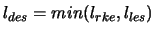
$Y_k = \rho \epsilon$ Similarly to the Spalart-Allmaras model, the delayed concept can be applied as well to the Realizable DES model to preserve the RANS mode throughout the boundary layer. The DES length $l_{des}$ in Equation  4.10-8 is redefined such that