4.7.2 Transport Equations for the Transition SST Model

The transport equation for the intermittency $\gamma$ is defined as:

The transition sources are defined as follows:

$$P_{\gamma 1} = 2F_{length}\rho S[\gamma F_{onset}]^{c_{\gamma 3}}$$

$$E_{\gamma 1} = P_{\gamma 1} \gamma$$ (4.7-2)

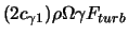
where $S$ is the strain rate magnitude. $F_{length}$ is an empirical correlation that controls the length of the transition region. The destruction/relaminarization sources are defined as follows:

$$P_{\gamma 2} = (2c_{\gamma 1})\rho \Omega \gamma F_{turb}$$

$$E_{\gamma 2} = c_{\gamma 2} P_{\gamma 2} \gamma$$ (4.7-3)

where $\Omega$ is the vorticity magnitude. The transition onset is controlled by the following functions:

$$Re_V = \frac{\rho y^2 S}{\mu}$$

$$R_T = \frac{\rho k}{\mu \omega}$$ (4.7-4)

$$F_{onset 1} = \frac{Re_v}{2.193 Re_{\theta c}}$$

$$F_{onset 2} = min(max(F_{onset 1}, F_{onset 1}^4),2.0)$$ (4.7-5)

$$F_{onset 3} = max\left(1-\left(\frac{R_T}{2.5}\right) ^3, 0\right)$$

$$F_{onset} = max(F_{onset 2} - F_{onset 3}, 0)$$

$$F_{turb} = e^{-\left(\frac{R_T}{4}\right)^4}$$ (4.7-6)

$Re_{\theta c}$ is the critical Reynolds number where the intermittency first starts to increase in the boundary layer. This occurs upstream of the transition Reynolds number $\widetilde{Re_{\theta t}}$ and the difference between the two must be obtained from an empirical correlation. Both the $F_{length}$ and $Re_{\theta c}$ correlations are functions of $\widetilde{Re_{\theta t}}$.

The constants for the intermittency equation are:

Separation Induced Transition Correction

The modification for separation-induced transition is:

$$\gamma_{sep} = min\left(2 max\left[ \left(\frac{Re_v}{3.235 Re_{\theta c}}\right) -1,0\right] F_{reattch},2\right) F_{\theta t}$$

$$F_{reattch} = e^{-\left(\frac{R_T}{20}\right)^4}$$

$$\gamma_{eff} = max(\gamma,\gamma_{sep})$$ (4.7-7)

The model constants in Equation  4.7-7 have been adjusted from those of Menter et al. [ 226] in order to improve the predictions of separated flow transition. The main difference is that the constant that controls the relation between $Re_v$ and $Re_{\theta c}$ was changed from 2.193, its value for a Blasius boundary layer, to 3.235, the value at a separation point where the shape factor is 3.5 [ 226]. The boundary condition for $\gamma$ at a wall is zero normal flux, while for an inlet, $\gamma$ is equal to 1.0.

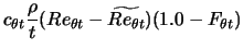
The transport equation for the transition momentum thickness Reynolds number $\widetilde{Re_{\theta t}}$ is

The source term is defined as follows:

$$P_{\theta t} = c_{\theta t} \frac{\rho}{t}(Re_{\theta t} - \widetilde{Re_{\theta t}})(1.0 - F_{\theta t})$$

$$t = \frac{500 \mu}{\rho U^2}$$ (4.7-9)

$$\theta_{BL} = \frac{\widetilde{Re_{\theta t}}\mu}{\rho U}$$

$$\delta_{BL} = \frac{15}{2}\theta_{BL}$$ (4.7-11)

$$\delta = \frac{50 \Omega y}{U}\delta_{BL}$$

$$Re_{\omega} = \frac{\rho \omega y^2}{\mu}$$

$$F_{wake} = e^{-\left(\frac{Re_{\omega}}{1E+5}\right)^2}$$ (4.7-12)

The model constants for the $\widetilde{Re_{\theta t}}$ equation are:

The boundary condition for $\widetilde{Re_{\theta t}}$ at a wall is zero flux. The boundary condition for $\widetilde{Re_{\theta t}}$ at an inlet should be calculated from the empirical correlation based on the inlet turbulence intensity.

The model contains three empirical correlations. $Re_{\Theta t}$ is the transition onset as observed in experiments. This has been modified from Menter et al. [ 226] in order to improve the predictions for natural transition. It is used in Equation  4.7-9. $F_{length}$ is the length of the transition zone and is substituted in Equation  4.7-2. $Re_{\Theta c}$ is the point where the model is activated in order to match both $Re_{\Theta t}$ and $F_{length}$, and is used in Equation  4.7-5. At present, these empirical correlations are proprietary and are not given in this manual.

$$Re_{\Theta t} = f(Tu,\lambda)$$

$$F_{length} = f(\widetilde{Re_{\Theta t}})$$

$$Re_{\Theta c} = f(\widetilde{Re_{\Theta t}})$$ (4.7-13)

The first empirical correlation is a function of the local turbulence intensity, $Tu$, and the Thwaites' pressure gradient coefficient $\lambda_{\theta}$ is defined as

where $dU/ds$ is the acceleration in the streamwise direction.

Coupling the Transition Model and SST Transport Equations

The transition model interacts with the SST turbulence model, as follows:

where $P_k$ and $D_k$ are the original production and destruction terms for the SST model and $F_{1orig}$ is the original SST blending function. Note that the production term in the $\omega$-equation is not modified. The rationale behind the above model formulation is given in detail in Menter et al. [ 226].

In order to capture the laminar and transitional boundary layers correctly, the mesh must have a $y^+$ of approximately one. If the $y^+$ is too large (i.e. $>$ 5), then the transition onset location moves upstream with increasing $y^+$. It is recommended to use the bounded second order upwind based discretization for the mean flow, turbulence and transition equations.