ANSYS FLUENT 12.0 Theory Guide - 16.7.4 Cavitation Models

16.7.4 Cavitation Models

A liquid at constant temperature can be subjected to a decreasing pressure, which may fall below the saturated vapor pressure. The process of rupturing the liquid by a decrease of pressure at constant temperature is called cavitation. The liquid also contains the micro-bubbles of noncondensable (dissolved or ingested) gases, or nuclei, which under decreasing pressure may grow and form cavities. In such processes, very large and steep density variations happen in the low-pressure/cavitating regions.

This section provides information about the following three cavitation models used in ANSYS FLUENT.

Singhal et al. model: You can use this model to include cavitation effects in two-phase flows when the mixture model is used. This is also known as the Full Cavitaton Model, which has been implemented in ANSYS FLUENTsince Version 6.1.
Zwart-Gerber-Belamri model: You can use this model in both the mixture and Eulerian multiphase models.
Schnerr and Sauer model: This is the default model. You can use this model in both the mixture and Eulerian multiphase models.

The following assumptions are made in the standard two-phase cavitation models:

The system under investigation must consist of a liquid and a vapor phase.
Mass transfer between the liquid and vapor phase is assumed to take place. Both bubble formation (evaporation) and collapse (condensation) are taken into account in the cavitation models.
The cavitation models are based on the Rayleigh-Plesset equation, describing the growth of a single vapor bubble in a liquid.
In the Singhal et al. model, noncondensable gases have been introduced into the system. The mass fraction of the noncondensable gases is assumed to be a known constant.
The input material properties used in the cavitation models can be constants, functions of temperature or user-defined.

The cavitation models offer the following capabilities:

The Singhal et al. model can be used to account for the effect of noncondensable gases. The Zwart-Gerber-Belamri and Schnerr and Sauer models do not include the noncondensable gases in the basic model terms.
The Zwart-Gerber-Belamri and Schnerr and Sauer models are compatible with all the turbulence models available in ANSYS FLUENT.
Both the pressure-based segregated and coupled solvers are available with the cavitation models.
They are all fully compatible with dynamic mesh and non-conformal interfaces.
Both liquid and vapor phases can be incompressible or compressible. For compressible liquids, the density is described using a user-defined function. See the separate UDF Manual for more information on user-defined density functions.

Limitations of the Cavitation Models

The following limitations apply to the cavitation models in ANSYS FLUENT:

None of the cavitation models can be used with the VOF model because the surface tracking schemes for the VOF model are incompatible with the interpenetrating continua assumption of the cavitation models.
They can only be used for cavitating flows occurring in a single liquid fluid.
The Singhal et al. model requires the primary phase to be a liquid and the secondary phase to be a vapor. This model is only compatible with the multiphase mixture model.
The Singhal et al. model cannot be used with the Eulerian multiphase model.
The Singhal et al. model is not compatible with the LES turbulence model.
The Zwart-Gerber-Belamri and Schnerr and Sauer models do not take the effect of noncondensable gases into account by default.

Vapor Transport Equation

With the multiphase cavitation modeling approach, a basic two-phase cavitation model consists of using the standard viscous flow equations governing the transport of mixture (Mixture model) or phases (Eulerian multiphase), and a conventional turbulence model (k- $\epsilon$ model). In cavitation, the liquid-vapor mass transfer (evaporation and condensation) is governed by the vapor transport equation:

$\frac{\partial}{\partial t}(\rm\alpha \rho_{v}) + \nabla. (\rm\alpha \rho_{v} \vec{V}_{v}) = R_{e} - R_{c}$

(16.7-12)

where,

	=	vapor phase
$\alpha$	=	vapor volume fraction
$\rho_{v}$	=	vapor density
$\vec{V}_{v}$	=	vapor phase velocity
$R_{e}$ , $R_{c}$	=	mass transfer source terms connected to the growth and collapse of the vapor bubbles repectively

In Equation 16.7-12, the terms $R_{e}$ and $R_{c}$ account for the mass transfer between the vapor and liquid phases in cavitation. In ANSYS FLUENT, they are modeled based on the Rayleigh-Plesset equation describing the growth of a single vapor bubble in a liquid.

Bubble Dynamics Consideration

In most engineering situations we assume that there are plenty of nuclei for the inception of cavitation. Thus, our primary focus is on proper accounting of bubble growth and collapse. In a flowing liquid with zero velocity slip between the fluid and bubbles, the bubble dynamics equation can be derived from the generalized Rayleigh-Plesset equation as [ 37]

$\Re_{B}\frac{D^{2} \Re_{B}}{D t^{2}} + \frac{3}{2}(\frac{D \... ..._{\ell}}{\Re_{B}} \Re_{B} - \frac{2 S}{\rm\rho_{\ell} \Re_{B}}$

(16.7-13)

where,

$\Re_{B}$	=	bubble radius
$\sigma$	=	liquid surface tension coefficient
$\rho_{\ell}$	=	liquid density
$P_{B}$	=	bubble surface pressure
	=	local far-field pressure

Neglecting the second-order terms and the surface tension force, Equation 16.7-13 is simplified to

$\frac{D \Re_{B}}{D t} = \sqrt{\frac{2}{3} \frac{P_{B} - P}{\rho_{\ell}}}$

(16.7-14)

This equation provides a physical approach to introduce the effects of bubble dynamics into the cavitation model. It can also be considered to be an equation for void propagation and, hence, mixture density.

Singhal et al. Model

This cavitation model is based on the "full cavitation model", developed by Singhal et al. [ 318]. It accounts for all first-order effects (i.e., phase change, bubble dynamics, turbulent pressure fluctuations, and noncondensable gases). It has the capability to account for multiphase (N-phase) flows or flows with multiphase species transport, the effects of slip velocities between the liquid and gaseous phases, and the thermal effects and compressibility of both liquid and gas phases. The cavitation model can be used with the mixture multiphase model, with or without slip velocities. However, it is always preferable to solve for cavitation using the mixture model without slip velocity; slip velocities can be turned on if the problem suggests that there is significant slip between phases.

To derive an expression of the net phase change rate, Singhal et al. [ 318] uses the following two-phase continuity equations:

Liquid phase:

$\frac{\partial}{\partial t}[\displaystyle (1 - \alpha) \rho_... ... \nabla. [\displaystyle (1 - \alpha) \rho_{\ell} \vec{V}] = -R$

(16.7-15)

Vapor phase:

$\frac{\partial}{\partial t}(\displaystyle \alpha \rho_{v}) + \nabla. (\displaystyle \alpha \rho_{v} \vec{V}) = R$

(16.7-16)

Mixture:

$\frac{\partial}{\partial t}(\rho) + \nabla. (\rho \vec{V}) = 0$

(16.7-17)

where,

$\ell$	=	liquid phase
$\rho$	=	mixture density (function of phase volume fraction and density)

Mixture density $\rho$ is defined as

$\displaystyle \rho = \displaystyle \alpha \rho_{v} + \displaystyle (1 - \alpha) \displaystyle \rho_{\ell}$

(16.7-18)

Combining Equations 16.7-15, 16.7-16, and 16.7-17 yields a relationship between the mixture density and vapor volume fraction ( $\alpha$ ):

$\frac{D \rho}{D{t}} = - \displaystyle (\rho_{\ell} - \rho_{v}) \frac{D \alpha}{Dt}$

(16.7-19)

The vapor volume fraction ( $\alpha$ ) can be related to the bubble number density ( ) and the radius of bubble ( $\Re_{B}$ ) as

$\alpha = n \times (\frac{4}{3} \pi {\Re_{B}}^{3})$

(16.7-20)

Substituting Equation 16.7-20 into Equation 16.7-19 gives the following:

$\frac{D \rho}{Dt} = - \displaystyle (\rho_{\ell} - \rho_{v})... ... \displaystyle {(3 \alpha)}^{\frac{2}{3}} \frac{D \Re_{B}}{Dt}$

(16.7-21)

Using the Equation 16.7-14, and combining Equations 16.7-15, 16.7-16, 16.7-19, and 16.7-21, the expression for the net phase change rate ( ) is finally obtained as

$R = {\displaystyle (n 4 \pi)}^{\frac{1}{3}} \displaystyle {(... ... {[\frac{2}{3} (\frac{P_{B} - P}{\rho_{\ell}})]}^{\frac{1}{2}}$

(16.7-22)

Here represents the vapor generation or evaporation rate, i.e. the source term $R_{e}$ in Equation 16.7-12. All terms, except , are either known constants or dependent variables. In the absence of a general model for estimation of the bubble number density, the phase change rate expression is rewritten in terms of bubble radius ( $\Re_{B}$ ), as follows:

$R = \frac{3 \displaystyle \alpha}{\Re_{B}} \displaystyle \fr... ...ell}}{\rho} \sqrt{\frac{2}{3} \frac{(P_{B} - P)}{\rho_{\ell}}}$

(16.7-23)

Equation 16.7-23 indicates that the unit volume mass transfer rate is not only related to the vapor density ( $\rho_{v}$ ), but the function of the liquid density ( $\rho_{\ell}$ ), and the mixture density ( $\rho$ ) as well. Since Equation 16.7-23 is derived directly from phase volume fraction equations, it is exact and should accurately represent the mass transfer from liquid to vapor phase in cavitation (bubble growth or evaporation). As for bubble collapse or the condensation process, though it is expected to be different from that of bubble growth, Equation 16.7-23 is, as a first approximation, also often used to model the bubble collapse by using the absolute value of the pressure difference and treating the right side as a sink term.

It may be noted that in practical cavitation models, the local far-field pressure is usually taken to be the same as the cell center pressure. The bubble pressure $P_{B}$ is equal to the saturation vapor pressure in the absence of dissolved gases, mass transport and viscous damping, i.e., $P_{B}=P_{v}$ .

where,

$P_{B}$	=	bubble pressure
$P_{v}$	=	saturation vapor pressure

Based on Equation 16.7-23, Singhal et al. [ 394] proposed a model where the vapor mass fraction is the dependent variable in the transport equation. This model accommodates also a single phase formulation where the governing equations is given by:

$\frac{\partial}{\partial t} \displaystyle (f_{v} \rho) + \na... ...splaystyle (\Gamma \nabla \displaystyle f_{v}) + R_{e} - R_{c}$

(16.7-24)

where,

$f_{v}$	=	vapor mass fraction
$f_{g}$	=	noncondensable gases
$\Gamma$	=	diffusion coefficient

The rates of mass exchange are given by the following equations:

If $P \leq P_{v}$

$R_{e} = F_{vap} \displaystyle \frac{max (1.0 , \sqrt{k}) \di... ...sqrt{\frac{2}{3} \displaystyle \frac{(P_{v} - P)}{\rho_{ell}}}$

(16.7-25)

If $P \> P_{v}$

$R_{c} = F_{cond} \displaystyle \frac{max (1.0 , \sqrt{k}) f_... ...o_{l} \rho_{l} \sqrt{\frac{2}{3} \frac{(P_{v} - P)}{\rho_{l}}}$

(16.7-26)

The saturation pressure is corrected by an estimation of the local values of the turbulent pressure fluctuations:

$P_{v} = P_{sat} + \frac{1}{2}(0.39 k)$

(16.7-27)

The constants have the values $F_{vap} = 0.02$ and $F_{cond} = 0.01$ . In this model, the liquid-vapor mixture is assumed to be compressible. Also, the effects of turbulence and the noncondensable gases have been taken into account.

Zwart-Gerber-Belamri Model

Assuming that all the bubbles in a system have the same size, Zwart-Gerber-Belamri [ 395] proposed that the total interphase mass transfer rate per unit volume ( ) is calculated using the bubble density numbers ( ), and the mass change rate of a single bubble:

$R = n \times (4 \pi {\Re_{B}}^2 \rho_{v} \frac{D \Re_{B}}{D t})$

(16.7-28)

Substituting the value of in Equation 16.7-28 into Equation 16.7-20, we have the expression of the net mass transfer:

$R = \frac{3 \alpha \rho_{v}}{\Re_{B}}\sqrt{\frac{2}{3} \frac{P_{B} - P}{\rho_{\ell}}}$

(16.7-29)

Comparing Equations 16.7-29 and 16.7-23, you will notice that the difference is only in the density terms in the mass transfer rate. In Equation 16.7-29, the unit voume mass transfer rate is only related to the vapor phase density ( $\rho_{v}$ ). Unlike Equation 16.7-23, has no relation with the liquid phase and mixture densities in this model.

As in Equation 16.7-23, Equation 16.7-29 is derived assuming bubble growth (evaporation). To apply it to the bubble collapse process (condensation), the following generalized formulation is used:

$R_{e} = F\frac{3 \alpha \rho_{v}}{\Re_{B}}\sqrt{\frac{2}{3} \frac{\vert P_{B} - P\vert}{\rho_{\ell}}}sign(P_{B} -P)$

(16.7-30)

where is an empirical calibration coefficient. Though it is originally derived from evaporation, Equation 16.7-30 only works well for condensation. It is physically incorrect and numerically unstable if applied to evaporation. The fundamental reason is that one of the key assumptions is that the cavitation bubble does not interact with each other. This is plausible only during the earliest stage of cavitation when the cavitation bubble grows from the nucleation site. As the vapor volume fraction increases, the nucleation site density must decrease accordingly. 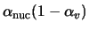To model this process, Zwart-Gerber-Belamri proposed to replace $\alpha_{v}$ with $\alpha_{\rm nuc}(1-\alpha_{v})$ in Equation 16.7-30. Then the final form of this cavitation model is as follows:

If $P \leq P_{v}$

$R_{e} = F_{\rm vap} \displaystyle \frac{3 \alpha_{\rm nuc} (... ...{v}}{\Re_{B}}\sqrt{\frac{2}{3} \frac{P_{v} - P}{\rho_{\ell}}}$

(16.7-31)

If $P \geq P_{v}$

$R_{c} = F_{\rm cond} \displaystyle \frac{3 \alpha_{v} \rho_{v}}{\Re_{B}}\sqrt{\frac{2}{3} \frac{P - P_{v}}{\rho_{\ell}}}$

(16.7-32)

where,

$\Re_{B}$	=	bubble radius	=	${10}^{-6} m$
$\alpha_{nuc}$	=	nucleation site volume fraction	=	$5 \times 10 ^{-4}$
$F_{\rm vap}$	=	evaporation coefficient	=
$F_{\rm cond}$	=	condensation coefficient	=

Schnerr and Sauer Model

As in the Singhal et al. model, Schnerr and Sauer [ 309] follow a similar approach to derive the exact expression for the net mass transfer from liquid to vapor. The equation for the vapor volume fraction has the general form:

$\frac{\partial}{\partial t} (\alpha \rho_{v}) + \nabla.(\alp... ...\vec{V}) = \frac{\rho_{v} \rho_{l}}{\rho} \frac{D \alpha}{D t}$

(16.7-33)

Here, the net mass source term is as follows:

$R = \frac{\rho_{v} \rho_{l}}{\rho} \frac{d \alpha}{d t}$

(16.7-34)

Unlike Zwart-Gerber-Belamri and Singhal et al., Schnerr and Sauer use the following expression to connect the vapor volume fraction to the number of bubbles per volume of liquid:

$\alpha = \frac{n_{b} \frac{4}{3} \pi {\Re_{B}}^{3}}{1 + n_{b} \frac{4}{3} \pi {\Re_{B}}^{3}}$

(16.7-35)

Following a similar approach to Singhal et al., they derived the following equation:

$R = \frac{\rho_{v} \rho_{l}}{\rho} \alpha (1 - \alpha) \frac{3}{\Re_{B}} \sqrt{\frac{2}{3} \frac{(P_{v} - P)}{\rho_{l}}}$

(16.7-36)

$\Re_{B} = {(\frac{\alpha}{1 - \alpha} \frac{3}{4 \pi} \frac{1}{n} )}^{\frac{1}{3}}$

(16.7-37)

where,

	=	mass transfer rate
$\Re_{B}$	=	bubble radius

Comparing Equation 16.7-36 with Equations 16.7-23 and 16.7-29, it is obvious that unlike the two previous models, the mass transfer rate in the Schnerr and Sauer model is proportional to $\alpha_{v}(1-\alpha_{v})$ . Moreover, the function $f (\alpha_{v}, \rho_{v}, \rho_{l}) = \frac{\rho_{v} \rho_{l}}{\rho} \alpha (1 - \alpha)$ has the interesting property that it approaches zero when $\alpha = 0$ and $\alpha = 1$ , and reaches the maximum in between. Also in this model, the only parameter which must be determined is the number of spherical bubbles per volume of liquid. If you assume that no bubbles are created or destroyed, the bubble number density would be constant. The initial conditions for the nucleation site volume fraction and the equilibrium bubble radius would therefore be sufficient to specify the bubble number density ( ) from Equation 16.7-35 and then the phase transition by Equation 16.7-36.

As in the two other models, Equation 16.7-36 is also used to model the condensation process. The final form of the model is as follows:

When $P_{v} \geq P$ ,

$R_{e} = \frac{\rho_{v} \rho_{l}}{\rho} \alpha (1 - \alpha) \... ...rt{\frac{2}{3} \frac{(P_{v} - P)}{\rho_{l}}} %%if P_{v} \geq P$

(16.7-38)

When $P_{v} \leq P$ ,

$R_{c} = \frac{\rho_{v} \rho_{l}}{\rho} \alpha (1 - \alpha) \... ...rt{\frac{2}{3} \frac{(P - P_{v})}{\rho_{l}}} %%if P_{v} \leq P$

(16.7-39)

Additional Guidelines for the Cavitation Models

In practical applications of a cavitation model, several factors greatly influence numerical stability. For instance, the high pressure difference between the inlet and exit, large ratio of liquid to vapor density, and large phase change rates between the liquid and vapor all have unfavorable effects on solution convergence. In addition, poor initial conditions very often lead to an unrealistic pressure field and unexpected cavitating zones, which, once present, are usually difficult to correct. You may consider the following factors/tips when choosing a cavitation model and addressing potential numerical problems:

Choice of the cavitation models
In ANSYS FLUENT, there are three available cavitation models. The Zwart-Gerber-Belamri and the Schnerr and Sauer models have been implemented following an entirely different numerical procedure from the Singhal et al. model developed in ANSYS FLUENT 6.1. Numerically, these two models are robust and converge quickly. It is therefore highly recommended that you should use the Schnerr and Sauer or the Zwart-Gerber-Bleamri model. The Singhal et al. model, though physically similar to the other two, is numerically less stable and more difficult to use.
Choice of the solvers
In ANSYS FLUENT, both the segregated (SIMPLE, SIMPLEC, and PISO) and coupled pressure-based solvers can be used in cavitation. As usual, the coupled solver is generally more robust and converges faster, particularly for cavitating flows in rotating machinery (liquid pumps, inducers, imprellers, etc). For fuel injector applications, however, the segregated solver also performs very well with the Schnerr and Sauer and the Zwart-Gerber-Belamri models.
As for the Singhal et al. model, since the coupled solver does not show any significant advantages, it is suggested that the segregated solver is used.
Initial conditions
Though no special initial condition settings are required, we suggest that the vapor fraction is always set to inlet values. The pressure is set close to the highest pressure among the inlets and outlets to avoid unexpected low pressure and cavitating spots. In gereral, the Schnerr and Sauer and Zwart-Gerber-Belamri models are robust enough so that there is no need for specific initial conditions. But in some very complicated cases, it may be beneficial to obtain a realistic pressure field before substantial cavities are formed. This can be achieved by obtaining a converged/near-converged solution for a single phase liquid flow, and then enabling the cavitation model. Again, the Singhal et al. model is much more sensitive to initial conditions. The above mentioned treatments are generally required.
Pressure discretization schemes
As for general multiphase flows, it is more desirable to use the following pressure discretization schemes in cavitation applications in this order:
- PRESTO!
- body force weighted
- second order
The standard and linear schemes generally are not very effective in complex cavitating flows and you should avoid using them.
Relaxation factors
- Schnerr and Sauer and Zwart-Gerber-Belamri models
  The default settings generally work well. To achieve numerical efficiency, however, the following values may be recommended:
  - The relaxation factor for vapor is 0.5 or higher unless the solution diverges or all the residuals oscillate excessively.
  - The density and the vaporization mass can be relaxed, but in general set them to 1.
  - For the segregated solver, the relaxation factor for pressure should be no less than the value for the momentum equations.
  - For the coupled solver, the default value for the Courant number (200) may need to be reduced to 20-50 in some complex 3D cases.
- Singhal et al. model
  In general, small relaxation factors are recommended for momentum equations, usually between 0.05 - 0.4. The relaxation factor for the pressure-correction equation should generally be larger than those for momentum equations, say in the range of 0.2 - 0.7. The density and the vaporization mass (source term in the vapor equation) can also be relaxed to improve convergence. Typically, the relaxation factor for density is set between the values of 0.3 and 1.0, while for the vaporization mass, values between 0.1 and 1.0 may be appropriate. For some extreme cases, even smaller relaxation factors may be required for all the equations.
Special tips for the Singal et al. model
- Noncondensable gases
  Noncondensable gases are usually present in liquids. Even a small amount (e.g., 15 ppm) of noncondensable gases can have significant effects on both the physical results and the convergence characteristics of the solution. A value of zero for the mass fraction of noncondensable gases should generally be avoided. In some cases, if the liquid is purified of noncondensable gases, a much smaller value (e.g., 10 $^{-8}$ ) may be used to replace the default value of 1.5 $\times 10^{-5}$ . In fact, higher mass fractions of the noncondensable gases may in many cases enhance numerical stability and lead to more realistic results. In particular, when the saturation pressure of a liquid at a certain temperature is zero or very small, noncondensable gases will play a crucial role both numerically and physically.
- Limits for dependent variables
  In many cases, setting the pressure upper limit to a reasonable value can help convergence greatly at the early stage of the solution. It is advisable to always limit the maximum pressure when possible. By default, ANSYS FLUENT sets the maximum pressure limit to 5.0 $\times 10^{10}$ Pascal.
- Relaxation factor for the pressure correction equation
  For cavitating flows, a special relaxation factor is introduced for the pressure correction equation. By default, this factor is set to 0.7, which should work well for most of the cases. For some very complicated cases, however, you may experience the divergence of the AMG solver. Under those circumstances, this value may be reduced to no less than 0.4. You can set the value of this relaxation factor by typing a text command. For more information, contact your ANSYS FLUENT support engineer.

Extended Cavitation Model Capabilites

When cavitation occurs, in many practical applications other gaseous species exist in the systems. For instance, in a ventilated supercavitating vehicle, air is injected into a liquid to stabilize or increase the cavitation along the vehicle surfaces. In some cases, the incoming flow is a mixture of a liquid and some gaseous species. To predict those types of cavitating flows, the basic two-phase cavitation model needs to be extended to a multiphase (N-phase) flow, or a multiphase species transport cavitation model.

Multiphase Cavitation Models

The multiphase cavitation models are the extensions of the three basic two-phase cavitation models to multiphase flows. In addition to the primary liquid and secondary vapor phase, more secondary gaseous phases can be included into the computational system under the following assumptions:

Mass transfer (cavitation) only occurs between the liquid and vapor phase.
The basic two-phase cavitation models are still used to model the phase changes between the liquid and vapor.
Only one secondary phase can be defined as compressible gas phase, while a user-defined density may be applied to all the phases.
In the Singhal et al. model, the predescribed noncondensable gases can be included in the system. To exclude noncondensable gases from the system, the mass fraction needs to be set to 0, and the noncondensable gas needs to be modeled by a separate compressible gas phase.
For noncavitating phase ( ), the general transport equation governing the vapor phase is the volume fraction equation in the Zwart-Gerber-Belamri and Schnerr and Sauer models, while in the Singhal et al. model, a mass transfer equation is solved and the vapor must be the second phase.

Multiphase Species Transport Cavitation Model

In some cases, there are several gas phase components in a system which can be considered compressible. Since only one compressible gas phase is allowed in the general multiphase approach, the multiphase species transport approach offers an option to handle these types of applications by assuming that there is one compressible gas phase with multiple species.

The detailed description of the multiphase species transport approach can be found in Section 16.8. The multiphase species transport cavitation model can be summarized as follows:

All the assumptions/limitations for the multiphase cavitation model apply here.
The primary phase can only be a single liquid.
All the secondary phases allow more than one species.
The mass transfer between a liquid and a vapor phase/species is modeled by the basic cavitation models.
The mass transfer between other phases or species are modeled with the standard mass transfer approach. In the standard model, zero constant rates should be chosen.
For the phases with multiple species, the phase shares the same pressure as the other phases, but each species has its own pressure (i.e., partial pressure). As a result, the vapor density and the pressure used in Equation 16.7-26 are the partial density and pressure of the vapor.

Previous: 16.7.3 UDF-Prescribed Mass Transfer
Up: 16.7 Modeling Mass Transfer
Next: 16.7.5 Evaporation-Condensation Model