2.3.1 The Multiple Reference Frame Model

Overview

The MRF model [ 209] is, perhaps, the simplest of the two approaches for multiple zones. It is a steady-state approximation in which individual cell zones can be assigned different rotational and/or translational speeds. The flow in each moving cell zone is solved using the moving reference frame equations (see Section  2.2). If the zone is stationary ( $\omega = 0$), the equations reduce to their stationary forms. At the interfaces between cell zones, a local reference frame transformation is performed to enable flow variables in one zone to be used to calculate fluxes at the boundary of the adjacent zone. The MRF interface formulation will be discussed in more detail in Section  2.3.1.

It should be noted that the MRF approach does not account for the relative motion of a moving zone with respect to adjacent zones (which may be moving or stationary); the mesh remains fixed for the computation. This is analogous to freezing the motion of the moving part in a specific position and observing the instantaneous flowfield with the rotor in that position. Hence, the MRF is often referred to as the "frozen rotor approach."

While the MRF approach is clearly an approximation, it can provide a reasonable model of the flow for many applications. For example, the MRF model can be used for turbomachinery applications in which rotor-stator interaction is relatively weak, and the flow is relatively uncomplicated at the interface between the moving and stationary zones. In mixing tanks, for example, since the impeller-baffle interactions are relatively weak, large-scale transient effects are not present and the MRF model can be used.

Another potential use of the MRF model is to compute a flow field that can be used as an initial condition for a transient sliding mesh calculation. This eliminates the need for a startup calculation. The multiple reference frame model should not be used, however, if it is necessary to actually simulate the transients that may occur in strong rotor-stator interactions, the sliding mesh model alone should be used (see Section  3.2).

Examples

For a mixing tank with a single impeller, you can define a rotating reference frame that encompasses the impeller and the flow surrounding it, and use a stationary frame for the flow outside the impeller region. An example of this configuration is illustrated in Figure  2.3.1. (The dashes denote the interface between the two reference frames.) Steady-state flow conditions are assumed at the interface between the two reference frames. That is, the velocity at the interface must be the same (in absolute terms) for each reference frame. The mesh does not move.

Figure 2.3.1: Geometry with One Rotating Impeller

You can also model a problem that includes more than one rotating reference frame. Figure  2.3.2 shows a geometry that contains two rotating impellers side by side. This problem would be modeled using three reference frames: the stationary frame outside both impeller regions and two separate rotating reference frames for the two impellers. (As noted above, the dashes denote the interfaces between reference frames.)

Figure 2.3.2: Geometry with Two Rotating Impellers

The MRF Interface Formulation

The MRF formulation that is applied to the interfaces will depend on the velocity formulation being used. The specific approaches will be discussed below for each case. It should be noted that the interface treatment applies to the velocity and velocity gradients, since these vector quantities change with a change in reference frame. Scalar quantities, such as temperature, pressure, density, turbulent kinetic energy, etc., do not require any special treatment, and thus are passed locally without any change.

Interface Treatment: Relative Velocity Formulation

In ANSYS FLUENT's implementation of the MRF model, the calculation domain is divided into subdomains, each of which may be rotating and/or translating with respect to the laboratory (inertial) frame. The governing equations in each subdomain are written with respect to that subdomain's reference frame. Thus, the flow in stationary and translating subdomains is governed by the equations in Section  1.2, while the flow in rotating subdomains is governed by the equations presented in Section  2.2.1.

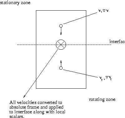
At the boundary between two subdomains, the diffusion and other terms in the governing equations in one subdomain require values for the velocities in the adjacent subdomain (see Figure  2.3.3). ANSYS FLUENT enforces the continuity of the absolute velocity, ${\vec v}$, to provide the correct neighbor values of velocity for the subdomain under consideration. (This approach differs from the mixing plane approach described in Section  2.3.2, where a circumferential averaging technique is used.)

When the relative velocity formulation is used, velocities in each subdomain are computed relative to the motion of the subdomain. Velocities and velocity gradients are converted from a moving reference frame to the absolute inertial frame using Equation  2.3-1.

Figure 2.3.3: Interface Treatment for the MRF Model

For a translational velocity $\vec{v_t}$, we have

From Equation  2.3-1, the gradient of the absolute velocity vector can be shown to be

Note that scalar quantities such as density, static pressure, static temperature, species mass fractions, etc., are simply obtained locally from adjacent cells.

Interface Treatment: Absolute Velocity Formulation

When the absolute velocity formulation is used, the governing equations in each subdomain are written with respect to that subdomain's reference frame, but the velocities are stored in the absolute frame. Therefore, no special transformation is required at the interface between two subdomains. Again, scalar quantities are determined locally from adjacent cells.