ANSYS FLUENT 12.0 Theory Guide - 16.5.4 Interphase Exchange Coefficients

16.5.4 Interphase Exchange Coefficients

It can be seen in Equations 16.5-13 and 16.5-14 that momentum exchange between the phases is based on the value of the fluid-fluid exchange coefficient $K_{pq}$ and, for granular flows, the fluid-solid and solid-solid exchange coefficients $K_{ls}$ .

Fluid-Fluid Exchange Coefficient

For fluid-fluid flows, each secondary phase is assumed to form droplets or bubbles. This has an impact on how each of the fluids is assigned to a particular phase. For example, in flows where there are unequal amounts of two fluids, the predominant fluid should be modeled as the primary fluid, since the sparser fluid is more likely to form droplets or bubbles. The exchange coefficient for these types of bubbly, liquid-liquid or gas-liquid mixtures can be written in the following general form:

$K_{pq} = \frac{\alpha_q \alpha_p \rho_p f}{\tau_p}$

(16.5-15)

where , the drag function, is defined differently for the different exchange-coefficient models (as described below) and $\tau_p$ , the "particulate relaxation time'', is defined as

$\tau_p = \frac{\rho_p d_p^2}{18 \mu_q}$

(16.5-16)

where is the diameter of the bubbles or droplets of phase .

Nearly all definitions of include a drag coefficient ( ) that is based on the relative Reynolds number ( ). It is this drag function that differs among the exchange-coefficient models. For all these situations, $K_{pq}$ should tend to zero whenever the primary phase is not present within the domain. To enforce this, the drag function is always multiplied by the volume fraction of the primary phase , as is reflected in Equation 16.5-15.

For the model of Schiller and Naumann [ 305]

$f = \frac{C_D {\rm Re}}{24}$ (16.5-17)

where

$C_D = \left\{ \begin{array}{ll} 24(1 + 0.15 \; {\rm Re}^{0.6... ...m Re} \leq 1000 \\ 0.44 & {\rm Re} > 1000 \end{array} \right.$ (16.5-18)

and Re is the relative Reynolds number. The relative Reynolds number for the primary phase and secondary phase is obtained from

${\rm Re} = \frac{ \rho_{q} \vert \vec v_p - \vec v_q\vert d_p }{\mu_q}$ (16.5-19)

The relative Reynolds number for secondary phases and is obtained from

${\rm Re} = \frac{ \rho_{rp} \vert \vec v_r- \vec v_p \vert d_{rp} }{\mu_{rp}}$ (16.5-20)

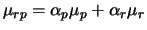where $\mu_{rp} = \alpha_p \mu_p+ \alpha_r \mu_r$ is the mixture viscosity of the phases and .
The Schiller and Naumann model is the default method, and it is acceptable for general use for all fluid-fluid pairs of phases.
For the Morsi and Alexander model [ 238]

$f = \frac{C_D {\rm Re}}{24}$ (16.5-21)

where

$C_D = a_1 + \frac{a_2}{\rm Re} + \frac{a_3}{{\rm Re}^2}$ (16.5-22)

and Re is defined by Equation 16.5-19 or 16.5-20. The 's are defined as follows:

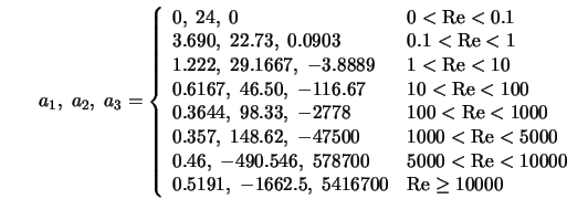$a_1, \; a_2, \; a_3 = \left\{ \begin{array}{ll} 0, \; 24, \;... ... -1662.5, \; 5416700 & {\rm Re} \geq 10000 \end{array} \right.$ (16.5-23)

The Morsi and Alexander model is the most complete, adjusting the function definition frequently over a large range of Reynolds numbers, but calculations with this model may be less stable than with the other models.
For the symmetric model

$K_{pq} = \frac{\alpha_p (\alpha_p \rho_p + \alpha_q \rho_q) f}{\tau_{pq}}$ (16.5-24)

where

$\tau_{pq} = \frac{(\alpha_p \rho_p + \alpha_q \rho_q) (\frac{d_p + d_q}{2})^2} {18 (\alpha_p \mu_p + \alpha_q \mu_q)}$ (16.5-25)

and

$f = \frac{C_D {\rm Re}}{24}$ (16.5-26)

where

$C_D = \left\{ \begin{array}{ll} 24(1 + 0.15 \; {\rm Re}^{0.6... ...m Re} \leq 1000 \\ 0.44 & {\rm Re} > 1000 \end{array} \right.$ (16.5-27)

and Re is defined by Equation 16.5-19 or 16.5-20. Note that if there is only one dispersed phase, then in Equation 16.5-25.
The symmetric model is recommended for flows in which the secondary (dispersed) phase in one region of the domain becomes the primary (continuous) phase in another. Thus for a single dispersed phase, and $\frac{(d_p+d_q)}{2} = d_p$ . For example, if air is injected into the bottom of a container filled halfway with water, the air is the dispersed phase in the bottom half of the container; in the top half of the container, the air is the continuous phase. This model can also be used for the interaction between secondary phases.

You can specify different exchange coefficients for each pair of phases. It is also possible to use user-defined functions to define exchange coefficients for each pair of phases. If the exchange coefficient is equal to zero (i.e., if no exchange coefficient is specified), the flow fields for the fluids will be computed independently, with the only "interaction'' being their complementary volume fractions within each computational cell.

Fluid-Solid Exchange Coefficient

The fluid-solid exchange coefficient $K_{sl}$ can be written in the following general form:

$K_{sl} = \frac{\alpha_s \rho_s f}{\tau_s}$

(16.5-28)

where is defined differently for the different exchange-coefficient models (as described below), and $\tau_s$ , the "particulate relaxation time'', is defined as

$\tau_s = \frac{\rho_s d_s^2}{18 \mu_l}$

(16.5-29)

where is the diameter of particles of phase .

All definitions of include a drag function ( ) that is based on the relative Reynolds number (Re ). It is this drag function that differs among the exchange-coefficient models.

For the Syamlal-O'Brien model [ 342]

$f = \frac{C_D {\rm Re}_s \alpha_l}{24 v_{r,s}^2}$ (16.5-30)

where the drag function has a form derived by Dalla Valle [ 66]

$C_D = \left(0.63 + \frac{4.8}{\sqrt{{\rm Re}_{s}/v_{r,s}}} \right)^2$ (16.5-31)

This model is based on measurements of the terminal velocities of particles in fluidized or settling beds, with correlations that are a function of the volume fraction and relative Reynolds number [ 294]:

${\rm Re}_{s} = \frac{\rho_l d_s \vert \vec v_s - \vec v_l \vert}{\mu_l}$ (16.5-32)

where the subscript is for the $l^{\rm th}$ fluid phase, is for the $s^{\rm th}$ solid phase, and is the diameter of the $s^{\rm th}$ solid phase particles.
The fluid-solid exchange coefficient has the form

$K_{sl} = \frac{3 \alpha_{s} \alpha_l \rho_l}{4 v_{r,s}^2 d_{... ...{\rm Re}_{s}}{v_{r,s}} \right) \vert \vec v_s - \vec v_l \vert$ (16.5-33)

where $v_{r,s}$ is the terminal velocity correlation for the solid phase [ 105]:

$v_{r,s} = 0.5 \left(A - 0.06 \; {\rm Re}_{s} + \sqrt{\left(... ...^2 + 0.12 \; {\rm Re}_{s} \left(2B - A \right) + A^2} \right)$ (16.5-34)

with

$A = \alpha_l^{4.14}$ (16.5-35)

and

$B = 0.8 \alpha_l^{1.28}$ (16.5-36)

for $\alpha_l \leq 0.85$ , and

$B = \alpha_l^{2.65}$ (16.5-37)

for $\alpha_l > 0.85$ .
This model is appropriate when the solids shear stresses are defined according to Syamlal et al. [ 343] (Equation 16.5-83).
For the model of Wen and Yu [ 373], the fluid-solid exchange coefficient is of the following form:

$K_{sl} = \frac{3}{4} C_D \frac{ \alpha_s \alpha_l \rho_l \vert \vec v_s - \vec v_l \vert }{d_s} \alpha_l^{-2.65}$ (16.5-38)

where

$C_D = \frac{24}{\alpha_l {\rm Re}_s} \left[ 1 + 0.15 (\alpha_l {\rm Re}_s)^{0.687} \right]$ (16.5-39)

and Re is defined by Equation 16.5-32.
This model is appropriate for dilute systems.
The Gidaspow model [ 110] is a combination of the Wen and Yu model [ 373] and the Ergun equation [ 88].
When $\alpha_l > 0.8$ , the fluid-solid exchange coefficient $K_{sl}$ is of the following form:

$K_{sl} = \frac{3}{4} C_D \frac{ \alpha_s \alpha_l \rho_l \vert \vec v_s - \vec v_l \vert }{d_s} \alpha_l^{-2.65}$ (16.5-40)

where

$C_D = \frac{24}{\alpha_l {\rm Re}_s} \left[ 1 + 0.15 (\alpha_l {\rm Re}_s)^{0.687} \right]$ (16.5-41)

When $\alpha_l \leq 0.8$ ,

$K_{sl} = 150\frac{\alpha_s (1-\alpha_l) \mu_l}{\alpha_l d_s^... ...5\frac{\rho_l \alpha_s \vert \vec v_s - \vec v_l \vert } {d_s}$ (16.5-42)

This model is recommended for dense fluidized beds.

Solid-Solid Exchange Coefficient

The solid-solid exchange coefficient $K_{ls}$ has the following form [ 341]:

$K_{ls} = \frac{ 3 \left(1 + e_{ls} \right) \left(\frac{\pi... ...+ \rho_{s} d_s^3 \right) } \vert \vec v_{l} - \vec v_{s} \vert$

(16.5-43)

where
	$e_{ls}$	=	the coefficient of restitution
	$C_{{\rm fr},ls}$	=	the coefficient of friction between the $l^{\rm th}$ and $s^{\rm th}$
			solid-phase particles $(C_{{\rm fr},ls} = 0)$
	$d_{l}$	=	the diameter of the particles of solid
	$g_{0,ls}$	=	the radial distribution coefficient

Note that the coefficient of restitution is described in Section 16.5.5 and the radial distribution coefficient is described in Section 16.5.5.

Universal Drag Laws for Bubble-Liquid and Droplet-Gas Flows

The universal drag laws [ 170] are suitable for the calculation of the drag coefficients in bubble-liquid or droplet-gas flow regimes. The drag laws can apply to non-spherical particles with the constraint of a pool flow regime, i.e. the hydraulic diameter of the flow domain which is far larger than the averaged size of the particles.

The exchange coefficient for bubbly and droplet flows can be written in the general form

$K_{pq} = \frac{\alpha_q \alpha_p \rho_p f}{\tau_p}$

(16.5-44)

Where represents the primary phase and the particulate phase. The particulate relaxation time $\tau_p$ is defined as

$\tau_p = \frac{\rho_p {d_p}^2}{18 \mu_e}$

(16.5-45)

The drag function is defined as

$f = \frac{C_D Re}{24}$

(16.5-46)

The relative Reynolds number for the primary phase and the secondary phase is obtained based on the relative velocity of the two phases.

$Re = \frac{\rho_q \vert\vec{v_q} - \vec{v_p}\vert d_p}{\mu_e}$

(16.5-47)

Where $\mu_e$ is the effective viscosity of the primary phase accounting for the effects of family of particles in the continuum.

The Rayleigh-Taylor instability wavelength is

$\lambda_{RT} = \left(\frac{\sigma}{g \Delta \rho_{pq}}\right)^{0.5}$

(16.5-48)

Where $\sigma$ is the surface tension, the gravity, and $\Delta \rho_{pq}$ the absolute value of the density difference between phases and .

The drag coefficient is defined differently for bubbly and droplet flows.

Bubble-Liquid Flow

$C_{D_{vis}} = \frac{24}{Re}(1+0.1Re^{0.75})$

(16.5-49)

$C_{D_{dis}} = 2/3(\frac{d_p}{\lambda_{RT}}){\left\lbrace\fra... ...}^{6/7}}{18.67{f^*}}\right\rbrace}^2;{f^*}=(1-\alpha_p)^{1.5}$

(16.5-50)

$C_{D_{cap}} = \frac{8}{3}(1-\alpha_p)^2$

(16.5-51)

In the viscous regime, the following condition is satisfied:

$C_{D_{dis}} < C_{D_{vis}}$ (16.5-52)

The drag coefficient, , is computed as

$C_D = C_{D_{vis}}$ (16.5-53)
In the distorted bubble regime, the following condition is satisfied:

$C_{D_{vis}} < C_{D_{dis}} < C_{D_{cap}}$ (16.5-54)

The drag coefficient is calculated as

$C_D = C_{D_{dis}}$ (16.5-55)
In the regime of strongly deformed, capped bubbles, the following condition is satisfied:

$C_{D_{dis}} > C_{D_{cap}}$ (16.5-56)

The drag coefficient can be written as

$C_D = C_{D_{cap}}$ (16.5-57)

The effective viscosity for the bubble-liquid mixture is

$\mu_e = \frac{\mu_q}{1-\alpha_p}$

(16.5-58)

Droplet-Gas Flow

When Re 1, the drag coefficient for the stokes regime is

$C_D = \frac{24}{Re}$ (16.5-59)
When 1 $\leq$ Re $\leq$ 1000, the drag coefficient for the viscous regime is

$C_D = \frac{24}{Re}(1+0.1Re^{0.75})$ (16.5-60)
For the Newton's regime (Re $\geq$ 1000), the drag coefficient is

$C_D = 2/3(\frac{d_p}{\lambda_{RT}}){\left\lbrace\frac{1+17.67{f^*}^{6/7}}{18.67{f^*}}\right\rbrace}^2;{f^*}=(1-\alpha_p)^3$ (16.5-61)

The effective viscosity for a bubble-liquid mixture is

$\mu_e = \frac{\mu_q}{({1-\alpha_p})^{2.5}}$

(16.5-62)

The drag model is currently suitable for bubble-liquid and/or droplet-gas flow when the characteristic length of the flow domain is much larger than the averaged size of the particles.

Previous: 16.5.3 Conservation Equations
Up: 16.5 Eulerian Model Theory
Next: 16.5.5 Solids Pressure