15.7.3 Splashing

If the particle impinging on the surface has a sufficiently high energy, the particle splashes and several new particles are created. You can explicitly set the number of particles created by each impact in the DPM tab of the Wall boundary condition dialog box. The number of splashed parcels may be set to an integer value between zero and ten. The properties (diameter, magnitude, and direction) of the splashed parcels are randomly sampled from the experimentally obtained distribution functions described in the following sections. Setting the number of splashed parcels to zero turns off the splashing calculation. Bear in mind that each splashed parcel can be considered a discrete sample of the distribution curves and that selecting the number of splashed drops in the Wall boundary condition dialog box does not limit the number of splashed drops, only the number of parcels representing those drops.

Therefore, for each splashed parcel, a different diameter is obtained by sampling a cumulative probability distribution function (CPDF), which is obtained from a Weibull distribution function and fitted to the data from Mundo, et al. [ 241]. The equation is

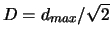and it represents the probability of finding drops of diameter $d_i$ in a sample of splashed drops. This distribution is similar to the Nakamura-Tanasawa distribution function used by O'Rourke [ 258], but with the peak of the distribution function being $D = d_{max}/\sqrt{2}$. To ensure that the distribution functions produce physical results with an increasing Weber number, the following expression for $d_{max}$ from O'Rourke [ 258] is used. The peak of the splashed diameter distribution is

where the expression for energy is given by Equation  15.7-1. Low Weber number impacts are described by the second term in Equation  15.7-5 and the peak of the minimum splashed diameter distribution is never less than 0.06 for very high energy impacts in any of the experiments analyzed by O'Rourke [ 258]. The Weber number in Equation  15.7-5 is defined using the relative velocity and drop diameter:

The cumulative probability distribution function (CPDF) is needed so that a diameter can be sampled from the experimental data. The CPDF is obtained from integrating Equation  15.7-4 to obtain

which is bounded by zero and one. An expression for the diameter (which is a function of $D$, the impingement Weber number $We$, and the impingement energy) is obtained by inverting Equation  15.7-7 and sampling the CPDF between zero and one. The expression for the diameter of the $i^{\rm th}$ splashed parcel is therefore given by,

where $c_i$ is the $i^{\rm th}$ random sample. Once the diameter of the splashed drop has been determined, the probability of finding that drop in a given sample is determined by evaluating Equation  15.7-4 at the given diameter. The number of drops per parcel can be expressed as a function of the total number of splashed drops:

where the $pdf_i$ is for the $i^{\rm th}$ sample. The values of $pdf_i$ are then normalized so that their sum is one. Both the number per parcel ( $N_i$) and the total number of splashed drops ( $N_{tot}$) is unknown, but an expression for $N_{tot}$ can be obtained from the conservation of mass if the total splashed mass is known.

The amount of mass splashed from the surface is a quadratic function of the splashing energy, obtained from the experimental data from Mundo [ 241]. The splashed mass fraction $y_s$ is given by

$$y_s = \left\{ \begin{array}{ll} 1.8 \mbox{x} 10^{-4} (E^2 - E^2_{crit} ) & ,E^2_{crit} < E^2 < 7500 \\ 0.70 & , E^2 > 7500 \end{array}\right.$$

The authors (O'Rourke et al. [ 258]) noted that nearly all of the impacts for typical diesel sprays are well above the upper bound and so the splashing event nearly always ejects 70% of the mass of the impinging drop. To obtain an expression for the total number of drops, we note that overall conservation of mass requires that the sum of the total mass of the splashed parcel(s) must equal the splashed mass fraction, or

where $m_0$ is the total mass of the impinging parcel. The expression for the total number of splashed drops is

The number of splashed drops per parcel is then determined by Equation  15.7-8 with the values of $pdf_i$ given by Equation  15.7-4.

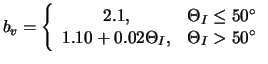
To calculate the velocity with which the splashed drops leave the surface, additional correlations are sampled for the normal component of the velocity. A Weibull function, fit to the data from Mundo [ 241], is used as the PDF for the normal component. The probability density is given by

where

$$b_v = \left\{ \begin{array}{cl} 2.1, & \Theta_I \leq 50^{\circ} \\ 1.10 + 0.02 \Theta_I, & \Theta_I > 50^{\circ} \end{array}\right.$$ (15.7-11)

and

where $\Theta_I$ is the angle at which the parcel impacts the surface, or the impingement angle. The tangential component of the velocity is obtained from the expression for the reflection angle $\Theta_s$:

combined with

Finally, an energy balance is performed for the new parcels so that the sum of the kinetic and surface energies of the new drops does not exceed that of the old drops. The energy balance is given by

where $E_{crit}$ is the threshold energy for splashing to occur. To ensure conservation of energy, the following correction factor is computed:

This correction factor is needed due to the relatively small number of sampled points for the velocity of the splashed drops (see Stanton [ 337] for more detail). The components of the splashed parcel are multiplied by the square root of $K$ in Equation  15.7-15 so that energy will be conserved. The normal and tangential velocity components of the splashed parcels are therefore given by

ANSYS FLUENT will limit the velocity of the splashed parcels so that they do not exceed the impact velocity of the original parcel. It is important to note that splashing events are inherently transient, so the splashing submodel is only available with unsteady tracking in ANSYS FLUENT. Splashing can also cause large increases in source terms in the cells in which it occurs, which can cause difficulty in convergence between time steps. Thus, it may be necessary to use a smaller time step during the simulation when splashing is enabled.