![[ANSYS, Inc. Logo]](fluentlogo.gif)


|
|
|
Proudman's Formula
Proudman [
280], using Lighthill's acoustic analogy, derived a formula for acoustic power generated by isotropic turbulence without mean flow. More recently, Lilley [
196] rederived the formula by accounting for the retarded time difference which was neglected in Proudman's original derivation. Both derivations yield acoustic power due to the unit volume of isotropic turbulence (in W/m
 ) as
) as
where
 and
and
 are the turbulence velocity and length scales, respectively, and
 is the speed of sound.
 in Equation
14.2-10 is a model constant. In terms of
in Equation
14.2-10 is a model constant. In terms of
 and
and
 , Equation
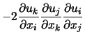
14.2-10 can be rewritten as
, Equation
14.2-10 can be rewritten as
 |
(14.2-11) |
where
 |
(14.2-12) |
 , is set to 0.1 in
ANSYS FLUENT based on the calibration of Sarkar and Hussaini [
301] using direct numerical simulation of isotropic turbulence.
, is set to 0.1 in
ANSYS FLUENT based on the calibration of Sarkar and Hussaini [
301] using direct numerical simulation of isotropic turbulence.
ANSYS FLUENT can also report the acoustic power in dB, which is computed from
where
 is the reference acoustic power (
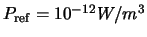 by default).
The Proudman's formula gives an approximate measure of the local contribution to total acoustic power per unit volume in a given turbulence field. Proper caution, however, should be taken when interpreting the results in view of the assumptions made in the derivation, such as high Reynolds number, small Mach number, isotropy of turbulence, and zero mean motion.
The Jet Noise Source Model
This source model for axisymmetric jets is based on the works of Goldstein [ 113] who modified the model originally proposed by Ribner [ 293] to better account for anisotropy of turbulence in axisymmetric turbulent jets.
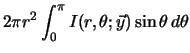
In Goldstein's model, the total acoustic power emitted by the unit volume of a turbulent jet is computed from
where
 and
and
 are the radial and angular coordinates of the receiver location, and
 is the directional acoustic intensity per unit volume of a jet defined by
 in Equation
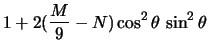
14.2-15 is the modified convection factor defined by
in Equation
14.2-15 is the modified convection factor defined by
 |
(14.2-16) |
 |
 |
 |
|
 |
![$\displaystyle \frac{1}{3}\left[\frac{M^2}{7} + M - 1.5 N (3 - 3 N + \frac{1.5}{\Delta^2} - \frac{\Delta^2}{2})\right] \, \sin^4 \theta$](img5538.gif) |
(14.2-17) | |
 |
 |
![$\displaystyle \cos^2 \theta \left[\cos^2 \theta + \frac{1}{2}\left(\frac{1}{\Delta^2} - 2 N\right) \sin^2 \theta\right]$](img5541.gif) |
(14.2-18) |
The remaining parameters are defined as
 |
 |
 |
(14.2-19) |
 |
 |
![$\displaystyle \left[\frac{3}{2}\left(\Delta -\frac{1}{\Delta}\right)\right]^2$](img5547.gif) |
(14.2-20) |
 |
 |
 |
(14.2-21) |
 |
 |
 |
(14.2-22) |
 |
 |
 |
(14.2-23) |
 |
 |
 |
(14.2-24) |
 and
and
 are computed differently depending on the turbulence model chosen for the computation. When the RSM is selected, they are computed from the corresponding normal stresses. For all other two-equation turbulence models, they are obtained from
 |
 |
 |
(14.2-25) |
 |
 |
 |
(14.2-26) |
ANSYS FLUENT reports the acoustic power both in the dimensional units (
 ) and in dB computed from
 is the reference acoustic power (
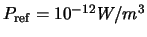 by default).
The Boundary Layer Noise Source Model
Far-field sound generated by turbulent boundary layer flow over a solid body at low Mach numbers is often of practical interest. The Curle's integral [ 64] based on acoustic analogy can be used to approximate the local contribution from the body surface to the total acoustic power. To that end, one can start with the Curle's integral
 denotes the emission time (
 ), and
 the integration surface.
Using this, the sound intensity in the far field can then be approximated by
 is the correlation area,
 , and
, and
 is the angle between
 and the wall-normal direction
 .
.
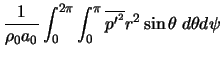
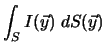
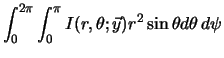
The total acoustic power emitted from the entire body surface can be computed from
 |
 |
 |
|
 |
 |
(14.2-30) |
ANSYS FLUENT reports the acoustic surface power defined by Equation
14.2-31 both in physical (
 ) and dB units.
Source Terms in the Linearized Euler Equations
The linearized Euler equations (LEE) can be derived from the Navier-Stokes equations starting from decompositions of the flow variables into mean, turbulent, and acoustic components, and by assuming that the acoustic components are much smaller than the mean and turbulent components. The resulting linearized Euler equations for the acoustic velocity components can be written as

 '' refers to the corresponding acoustic components, and the prime superscript refers to the turbulent components.
The right side of Equation
14.2-32 can be considered as effective source terms responsible for sound generation. Among them, the first three terms involving turbulence are the main contributors. The first two terms denoted by
 are often referred to as "shear-noise" source terms, since they involve the mean shear. The third term denoted by
 is often called the "self-noise" source term, as it involves turbulent velocity components only.
The turbulent velocity field needed to compute the LEE source terms is obtained using the method of stochastic noise generation and radiation (SNGR) [
23]. In this method, the turbulent velocity field and its derivatives are computed from a sum of
 Fourier modes.
 ,
,
 ,
,
 are the amplitude, phase, and directional (unit) vector of the
 Fourier mode associated with the wave-number vector
 .
.
Note that the source terms in the LEE are vector quantities, having two or three components depending on the dimension of the problem at hand.
Source Terms in Lilley's Equation
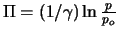
Lilley's equation is a third-order wave equation that can be derived by combining the conservation of mass and momentum of compressible fluids. When the viscous terms are omitted, it can be written in the following form:
where
 .
.
Lilley's equation can be linearized about the underlying steady flow as
 is the turbulent velocity component.
Substituting Equation
14.2-35 into the source term of Equation
14.2-34, we have
The resulting source terms in Equation 14.2-36 are evaluated using the mean velocity field and the turbulent (fluctuating) velocity components synthesized by the SNGR method. As with the LEE source terms, the source terms in Equation 14.2-36 are grouped depending on whether the mean velocity gradients are involved ( shear noise or self noise), and reported separately in ANSYS FLUENT.
Previous:
14.2.1 The Ffowcs Williams








![\overline{p'^2} \approx \frac{1}{16 \pi^2 a_0^2} \int_S \fra... ...{\vec y},\tau)\right]^2} {\cal A}_c ({\vec y}) \; dS({\vec y})](img5576.gif)
![I(\vec{y}) \equiv \frac{{\cal A}_c(\vec{y})}{12 \rho_0 \pi a_0^3} \overline{\left[\frac{\partial p}{\partial t}\right]^2}](img5587.gif)