Step 7: Postprocessing

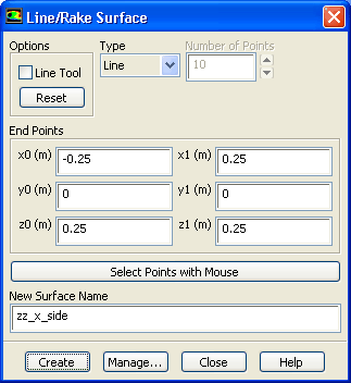
1.   Create the new surface, zz_x_side.

Surface $\rightarrow$ Line/Rake...

(a)   Enter (-0.25, 0, 0.25) for (x0, y0, z0) respectively.

(b)   Enter (0.25, 0, 0.25) for (x1, y1, z1) respectively.

(c)   Enter zz_x_side for New Surface Name.

(d)   Click Create and close the Line/Rake Surface dialog box.

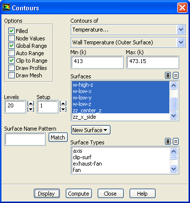
2.   Display contours of wall temperature (outer surface).

Graphics and Animations Contours Set Up...

(a)   Make sure that Filled is enabled in the Options group box.

(b)   Disable Node Values.

(c)   Select Temperature... and Wall Temperature (Outer Surface) from the Contours of drop-down lists.

(d)   Select all surfaces except default-interior and zz_x_side.

(e)   Disable Auto Range and Draw Mesh.

(f)   Enter 413 for Min and 473.15 for Max.

(g)   Click Display and rotate the view as shown in Figure  5.5.

Figure 5.5: Contours of Wall Temperature

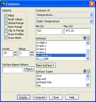
3.   Display contours of static temperature.

Graphics and Animations Contours Set Up...

(a)   Make sure that Filled is enabled in the Options group box.

(b)   Select Temperature... and Static Temperature from the Contours of drop-down lists.

(c)   Deselect all surfaces and select zz_center_z from the Surfaces selection list.

(d)   Enable Draw Mesh in the Options group box to open the Mesh Display dialog box.

i.   Make sure that Outline in the Edge Type list is selected.

ii.   Click Display and close the Mesh Display dialog box.

(e)   Enable Node Values.

(f)   Disable Auto Range.

(g)   Enter 421 for Min and 473.15 for Max.

(h)   Click Display and rotate the view as shown in Figure  5.6.

Figure 5.6: Contours of Static Temperature

  The temperature field now ties in with expectations, displaying good stratification with disturbance at the walls.

4.   Display contours of radiation heat flux.

Graphics and Animations Contours Set Up...

(a)   Make sure that Filled is enabled in the Options group box.

(b)   Disable both Node Values and Draw Mesh in the Options group box.

(c)   Select Wall Fluxes... and Radiation Heat Flux from the Contours of drop-down list.

(d)   Select all surfaces except default-interior and zz_x_side.

(e)   Click Display and rotate the view as shown in Figure  5.7.

(f)   Close the Contours dialog box.

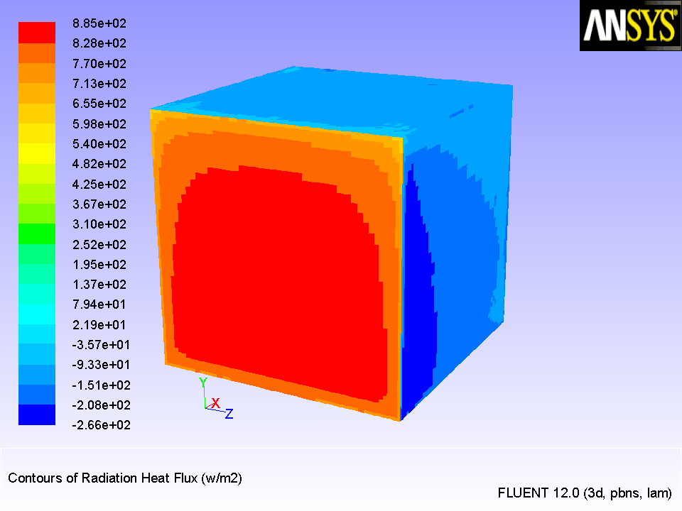
  Figure  5.7 shows the radiating wall ( w-low-x) with positive heat flux and all other walls with negative heat flux.

Figure 5.7: Contours of Radiation Heat Flux

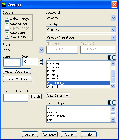
5.   Display vectors of velocity magnitude.

Graphics and Animations Vectors Set Up...

(a)   Retain the default selection of Velocity from the Vectors of drop-down list.

(b)   Retain the default selection of Velocity... and Velocity Magnitude from the Color by drop-down list.

(c)   Deselect all surfaces and select zz_center_z from the Surfaces selection list.

(d)   Enable Draw Mesh in the Options group box to open the Mesh Display dialog box.

i.   Make sure that Outline is selected in the Edge Type list.

ii.   Click Display and close the Mesh Display dialog box.

(e)   Enter 7 for Scale.

(f)   Click Display (Figure  5.8) and rotate the view as shown in Figure  5.8.

(g)   Close the Vectors dialog box.

Figure 5.8: Vectors of Velocity Magnitude

6.   Compute view factors and radiation emitted from the front wall ( w-high-x) to all other walls.

Report $\rightarrow$ S2S Information...

(a)   Make sure that View Factors is enabled in the Report Options group box.

(b)   Enable Incident Radiation.

(c)   Select w-high-x from the From selection list.

(d)   Select all zones except w-high-x from the To selection list.

(e)   Click Compute and close the S2S Information dialog box.

  The computed values of the Views Factors and Incident Radiation are displayed in the console. A view factor of approximately 0.2 for each wall is a good value for the square box.

7.   Compute the total heat transfer rate.

Reports Fluxes Set Up...

(a)   Select Total Heat Transfer Rate in the Options group box.

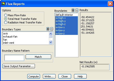
(b)   Select all boundary zones except default-interior from the Boundaries selection list.

(c)   Click Compute.

Note:   The energy imbalance is approximately 0.08%.

8.   Compute the total heat transfer rate for w-low-x.

Reports Fluxes Set Up...

(a)   Retain the selection of Total Heat Transfer Rate in the Options group box.

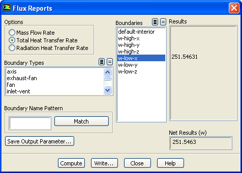
(b)   Deselect all boundary zones and select w-low-x from the Boundaries selection list.

(c)   Click Compute.

Note:   The net heat load is approximately 251.55 W

9.   Compute the radiation heat transfer rate..

Reports Fluxes Set Up...

(a)   Select Radiation Heat Transfer Rate in the Options group box.

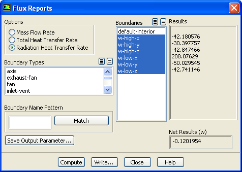
(b)   Select all boundary zones except default-interior from the Boundaries selection list.

(c)   Click Compute.

Note:   The net heat load is approximately -0.12 W.

10.   Compute the radiation heat transfer rate for w-low-x.

Reports Fluxes Set Up...

(a)   Retain the selection of Radiation Heat Transfer Rate in the Options group box.

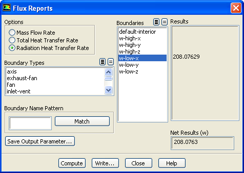
(b)   Deselect all boundary zones and select w-low-x from the Boundaries selection list.

(c)   Click Compute and close the Flux Reports dialog box.

  The net heat load is approximately 208.08 W. After comparing the total heat transfer rate and radiation heat transfer rate, it can be concluded that radiation is the dominant mode of heat transfer.

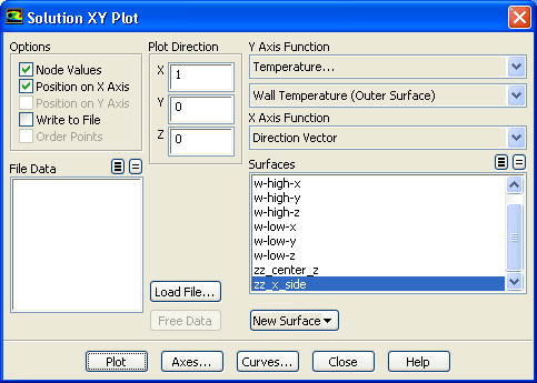
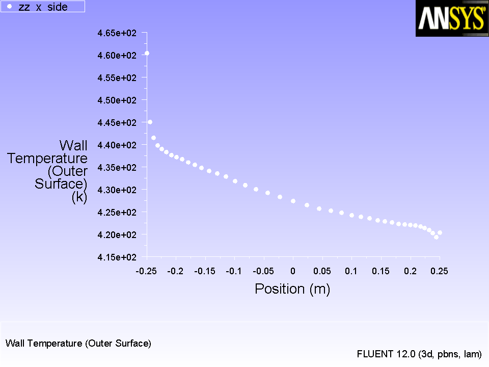
11.   Display temperature profile for the side wall.

Plots XY Plot Set Up...

(a)   Select Temperature... and Wall Temperature (Outer Surface) from the Y Axis Function drop-down lists.

(b)   Retain the default selection of Direction Vector from the X Axis Function drop-down list.

(c)   Select zz_x_side from the Surfaces selection list.

(d)   Click Plot (Figure  5.9).

(e)   Enable Write to File and click the Write... button to open the Select File dialog box.

i.   Enter tp_1.xy for XY File.

ii.   Click OK in the Select File dialog box.

(f)   Disable the Write to File option.

(g)   Close the Solution XY Plot dialog box.

Figure 5.9: Temperature Profile Along Side Wall

12.   Save the case and data files ( rad_b_1.cas.gz and rad_b_1.dat.gz).

File $\rightarrow$ Write $\rightarrow$ Case & Data...