Step 6: Solution

1.   Set the solution parameters.

Solution Methods

(a)   Select Body Force Weighted from the Pressure drop-down list in the Spatial Discretization group box.

(b)   Retain the default selection of First Order Upwind from the Momentum and Energy drop-down lists.

2.   Set the under-relaxation factors.

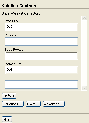
Solution Controls

(a)   Enter 0.4 for Momentum.

  Buoyancy driven cases will need stiffer relaxation for better results. A good starting point for momentum would be 0.4.

3.   Initialize the solution.

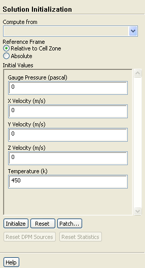
Solution Initialization

(a)   Enter 450 K for Temperature.

(b)   Click Initialize.

4.   Create the new surface, zz_center_z.

Surface $\rightarrow$ Iso-Surface...

(a)   Select Mesh... and Z-Coordinate from the Surface of Constant drop-down lists.

(b)   Click Compute and retain the value 0 in the Iso-Values field.

(c)   Enter zz_center_z for New Surface Name.

(d)   Click Create and close the Iso-Surface dialog box.

5.   Save the case file ( rad_a_1.cas.gz)

File $\rightarrow$ Write $\rightarrow$ Case...

6.   Start the calculation by requesting 100 iterations Figure  5.3.

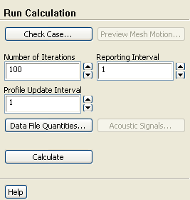
Run Calculation

(a)   Enter 100 for Number of Iterations.

(b)   Click Calculate.

Figure 5.3: Scaled Residuals

  An inspection of the residual plot at this stage suggests that the solution is not converging in a stable manner. This can be a common problem with natural convection (buoyancy driven) flows which tend to be unstable in their physical nature.

7.   Display contours of static temperature.

Graphics and Animations Contours Set Up...

(a)   Enable Filled in the Options group box.

(b)   Select Temperature... and Static Temperature from the Contours of drop-down lists.

(c)   Select zz_center_z from the Surfaces selection list.

(d)   Enable Draw Mesh in the Options group box to open the Mesh Display dialog box.

i.   Select Outline in the Edge Type list.

ii.   Click Display and close the Mesh Display dialog box.

(e)   Disable Auto Range.

(f)   Enter 421 for Min and 473.15 for Max.

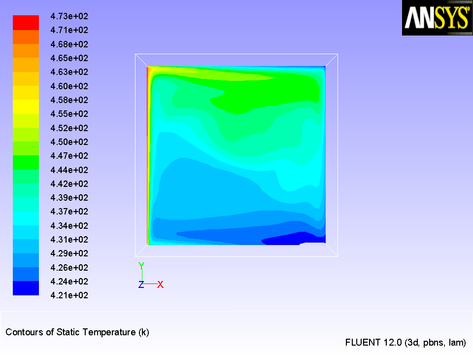
(g)   Click Display and rotate the view as shown in Figure  5.4.

(h)   Close the Contours dialog box. (Figure  5.4).

Figure 5.4: Contours of Static Temperature

  A regular check for most buoyant cases is to look for evidence of stratification in the temperature field, near horizontal bands of similar temperature. These may be broken or disturbed by buoyant plumes. For this case you can expect reasonable stratification with some disturbance at the vertical walls where the air is driven round. However, the results show very little evidence of this. This is most likely due to the physical instability of the flow process. To help overcome this, make use of relaxation to damp out the instabilities.

8.   Change the under-relaxation factor for Momentum.

Solution Controls

(a)   Enter 0.1 for Momentum.

  The relaxation factor on momentum was already reduced to 0.4 before solving. We shall now drop it even further to 0.1. In general, avoid this type of stiff relaxation as it will slow down the solution speed, but in cases like this it is necessary. However, avoid reducing the relaxation factor much further.

9.   Request 100 more iterations.

Run Calculation