Step 8: Compare the Contour Plots after Varying Radiating Surfaces

1.   Increase the number of faces per cluster to 10.

Models Radiation Edit...

(a)   Click the Set... button in the Parameters group box to open the View Factor and Cluster Parameters dialog box.

i.   Enter 10 for Faces per Surface Cluster for Flow Boundary Zones in the Parameters group box.

ii.   Click Apply to All Walls and close the View Factor and Cluster Parameters dialog box.

(b)   Click Compute/Write... for Methods in the View Factors group box to open the Select File dialog box and to compute the view factors.

  Specify a file name where the cluster and view factor parameters will be stored.

i.   Enter rad_10.s2s.gz for S2S File.

ii.   Click OK in the Select File dialog box.

(c)   Click OK to close the Radiation Model dialog box.

2.   Initialize the solution.

Solution Initialization

3.   Start the calculation by requesting 650 iterations.

Run Calculation

  The solution will converge in approximately 612 iterations.

4.   Save the case and data files ( rad_10.cas.gz and rad_10.dat.gz).

File $\rightarrow$ Write $\rightarrow$ Case & Data...

5.   In a manner similar to the steps described in Step 7: 11. (a)-(g), display the temperature profile for the side wall and write it to a file named tp_10.xy.

6.   Repeat the procedure outlined in Step 8: 1.-5. for 100, 400, 800, and 1600 faces per surface cluster and save the respective case and data files (e.g., rad_100.cas.gz) and temperature profile files (e.g., tp_100.xy).

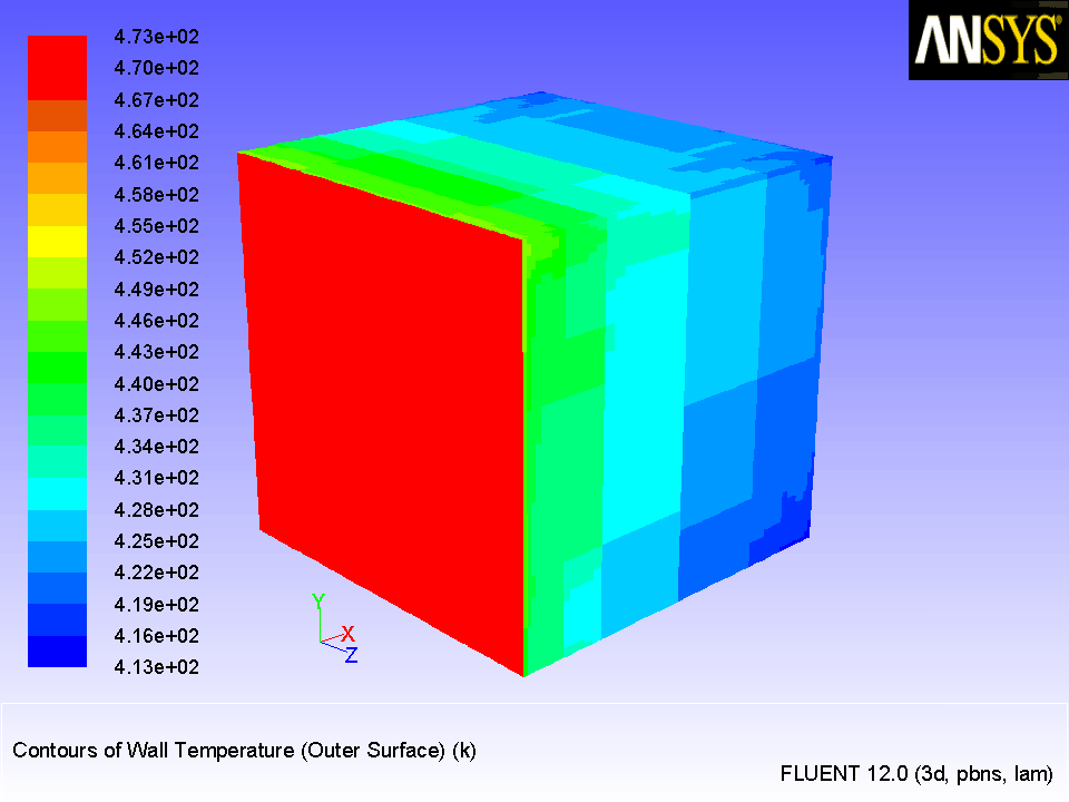
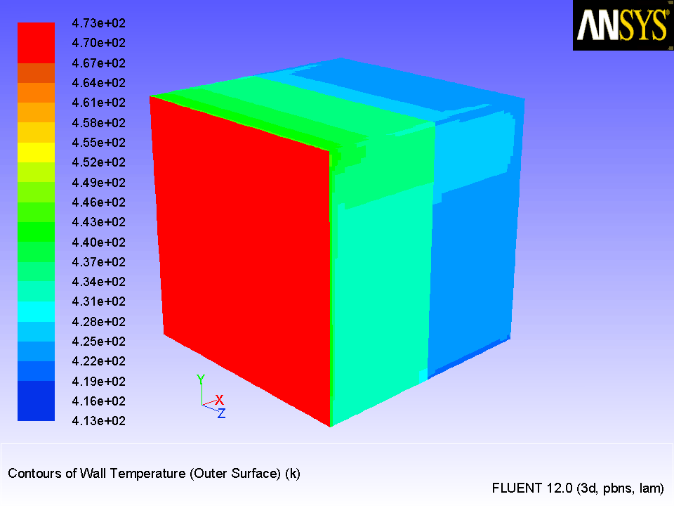
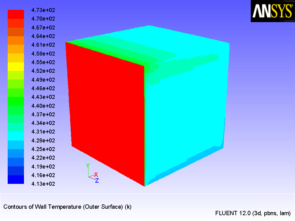
7.   Display contours of wall temperature (outer surface) for all six cases, in the manner described in Step 7: 2.

Graphics and Animations Contours Set Up...

Figure 5.10: Contours of Wall Temperature (Outer Surface): 1 Face per Surface Cluster

Figure 5.11: Contours of Wall Temperature (Outer Surface): 10 Faces per Surface Cluster

Figure 5.12: Contours of Wall Temperature (Outer Surface): 100 Faces per Surface Cluster

Figure 5.13: Contours of Wall Temperature (Outer Surface): 400 Faces per Surface Cluster

Figure 5.14: Contours of Wall Temperature (Outer Surface): 800 Faces per Surface Cluster

Figure 5.15: Contours of Wall Temperature (Outer Surface): 1600 Faces per Surface Cluster

8.   Display contours of surface cluster ID for 1600 faces per surface cluster (Figure  5.16).

Graphics and Animations Contours Set Up...

(a)   Make sure that Filled is enabled in the Options group box.

(b)   Make sure that Node Values is disabled.

(c)   Select Radiation... and Surface Cluster ID from the Contours of drop-down lists.

(d)   Select all surfaces except default-interior and zz_x_side.

(e)   Click Display and rotate the figure as shown in Figure  5.16.

(f)   Close the Contours dialog box.

Figure 5.16: Contours of Surface Cluster ID--1600 Faces per Surface Cluster (FPSC)

9.   Read rad_400.cas.gz and rad_400.dat.gz and, in a similar manner to the previous step, display contours of surface cluster ID (Figure  5.17).

Figure 5.17: Contours of Surface Cluster ID--400 FPSC

  Figure  5.17 shows contours of Surface Cluster ID for 400 FPSC. This case shows better clustering compared to all of the other cases.

10.   Display the temperature profile plot for 400 FPSC on a plot that includes the temperature profile plots for 1, 10, 100, 800, and 1600 FPSC.

Plots XY Plot Set Up...

(a)   Make sure that Write to File in the Options group is disabled.

(b)   Make sure that Temperature... and Wall Temperature (Outer Surface) are selected from the Y Axis Function drop-down lists.

(c)   Retain the default selection of Direction Vector from the X Axis Function drop-down list.

(d)   Make sure that zz_x_side is selected from the Surfaces selection list.

(e)   Click Plot (Figure  5.18).

(f)   Click the Load File... button to open the Select File dialog box.

i.   Select tp_1.xy.

ii.   Click OK to close the Select File dialog box.

(g)   Click Plot.

(h)   In a similar manner, click the Load File... button to read the files tp_10.xy, tp_100.xy, tp_800.xy, and tp_1600.xy, and plot the temperature profiles.

(i)   Close the Solution XY Plot dialog box.

Figure 5.18: A Comparison of Temperature Profiles along the Side Wall

Note:   The legend entries in Figure  5.18 have been changed for display purposes. You will see similar changes in Figure  5.19. You do not need to make these changes.