[ANSYS, Inc. Logo] return to home search
next up previous contents

Step 7: Solution: Steady Flow

  In this step, you will generate a steady-state flow solution that will be used as an initial condition for the time-dependent solution.

1.   Set the solution parameters.

figure Solution Methods

figure

(a)   Retain the default selection of Least Squares Cell Based from the Gradient drop-down list in the Spatial Discretization group box.

(b)   Select Second Order Upwind from the Turbulent Kinetic Energy and Specific Dissipation Rate drop-down lists.

  Second-order discretization provides optimum accuracy.

2.   Modify the Courant number.

figure Solution Controls

figure

(a)   Set the Courant Number to 50.

(b)   Retain the default values for the under-relaxation factors.

3.   Enable the plotting of residuals.

figure Monitors figure figure Residuals figure Edit...

figure

(a)   Make sure Plot is enabled in the Options group box.

(b)   Select none from the Convergence Criterion drop-down list.

(c)   Click OK to close the Residual Monitors dialog box.

4.   Enable the plotting of mass flow rate at the flow exit.

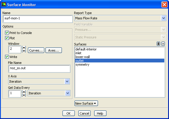
figure Monitors (Surface Monitors) figure Create...

figure

(a)   Enable Plot and Write.

Note:   When Write is enabled in the Surface Monitor dialog box, the mass flow rate history will be written to a file. If you do not enable the write option, the history information will be lost when you exit ANSYS FLUENT.

(b)   Enter noz_ss.out for File Name.

(c)   Select Mass Flow Rate in the Report Type drop-down list.

(d)   Select outlet in the Surfaces selection list.

(e)   Click OK to close the Surface Monitor dialog box.

5.   Save the case file ( noz_ss.cas).

File $\rightarrow$ Write $\rightarrow$ Case...

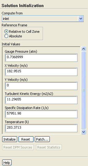
6.   Initialize the solution.

figure Solution Initialization

figure

(a)   Select inlet from the Compute from drop-down list.

(b)   Click Initialize.

7.   Perform gradient adaption to refine the mesh.

Adapt $\rightarrow$ Gradient...

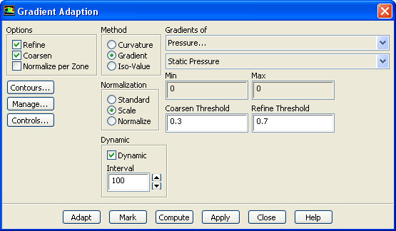
  You will enable dynamic adaption so that the solver periodically refines the mesh in the vicinity of the shocks as the iterations progress. The shocks are identified by their large pressure gradients.

figure

(a)   Select Gradient from the Method group box.

  The mesh adaption criterion can either be the gradient or the curvature (second gradient). Because strong shocks occur inside the nozzle, the gradient is used as the adaption criterion.

(b)   Select Scale from the Normalization group box.

  Mesh adaption can be controlled by the raw (or standard) value of the gradient, the scaled value (by its average in the domain), or the normalized value (by its maximum in the domain). For dynamic mesh adaption, it is recommended to use either the scaled or normalized value because the raw values will probably change strongly during the computation, which would necessitate a readjustment of the coarsen and refine thresholds. In this case, the scaled gradient is used.

(c)   Enable Dynamic in the Dynamic group box.

(d)   Enter 100 for the Interval.

  For steady-state flows, it is sufficient to only seldomly adapt the mesh--in this case an interval of 100 iterations is chosen. For time-dependent flows, a considerably smaller interval must be used.

(e)   Retain the default selection of Pressure... and Static Pressure from the Gradients of drop-down lists.

(f)   Enter 0.3 for Coarsen Threshold.

(g)   Enter 0.7 for Refine Threshold.

  As the refined regions of the mesh get larger, the coarsen and refine thresholds should get smaller. A coarsen threshold of 0.3 and a refine threshold of 0.7 result in a "medium'' to "strong'' mesh refinement in combination with the scaled gradient.

(h)   Click Apply to store the information.

(i)   Click the Controls... button to open the Mesh Adaption Controls dialog box.

figure

i.   Retain the default selection of fluid in the Zones selection list.

ii.   Enter 20000 for Max # of Cells.

  To restrict the mesh adaption, the maximum number of cells can be limited. If this limit is violated during the adaption, the coarsen and refine thresholds are adjusted to respect the maximum number of cells. Additional restrictions can be placed on the minimum cell volume, minimum number of cells, and maximum level of refinement.

iii.   Click OK to close the Mesh Adaption Controls dialog box.

(j)   Close the Gradient Adaption dialog box.

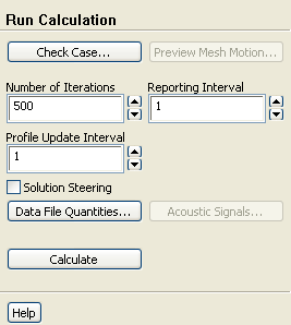
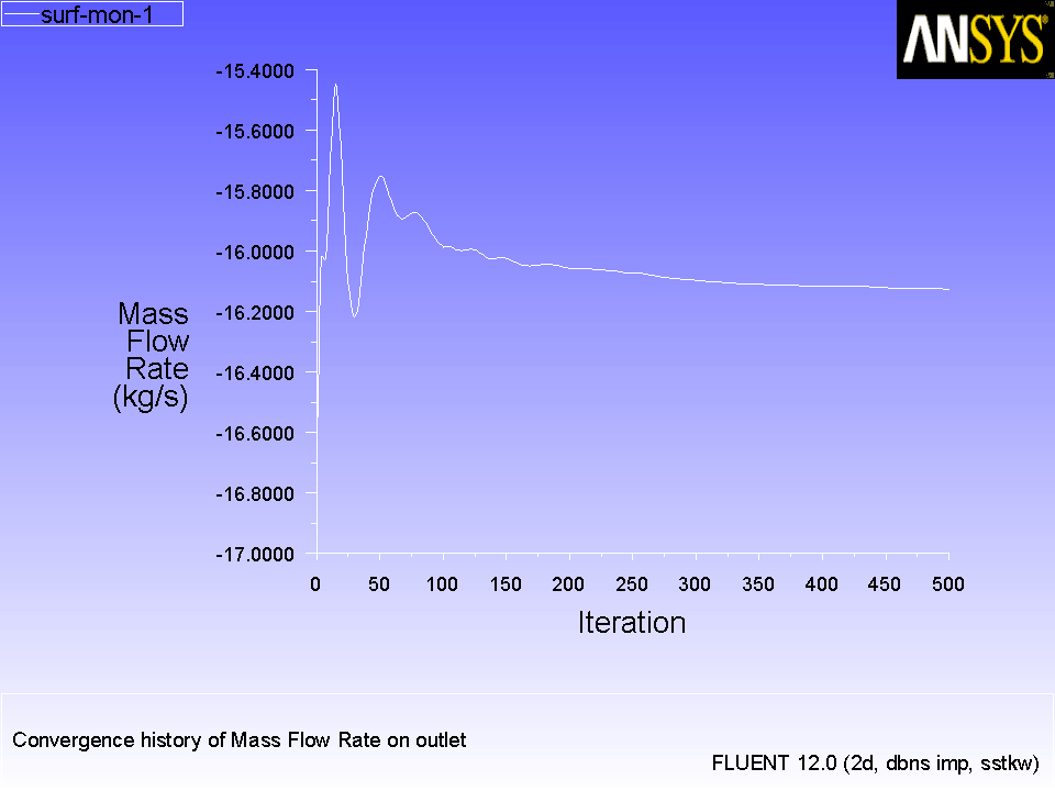
8.   Start the calculation by requesting 500 iterations.

figure Run Calculation

figure

Figure 4.3: Mass Flow Rate History
figure

9.   Save the case and data files ( noz_ss.cas and noz_ss.dat).

File $\rightarrow$ Write $\rightarrow$ Case & Data...

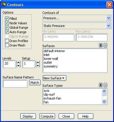
10.   Display the steady flow contours of static pressure (Figure  4.4).

figure Graphics and Animations figure figure Contours figure Set Up...

figure

(a)   Enable Filled in the Options group box.

(b)   Click Display and close the Contours dialog box.

Figure 4.4: Contours of Static Pressure (Steady Flow)
figure

  The steady flow prediction in Figure  4.4 shows the expected pressure distribution, with low pressure near the nozzle throat.

11.   Display the steady-flow velocity vectors (Figure  4.5).

figure Graphics and Animations figure figure Vectors figure Set Up...

figure

(a)   Retain all default settings.

(b)   Click Display and close the Vectors dialog box.

   You can zoom in to view the recirculation of your velocity vectors.

  The steady flow prediction in Figure  4.5 shows the expected form,with peak velocity of approximately 300 m/s through the nozzle.

Figure 4.5: Velocity Vectors (Steady Flow)
figure

12.   Check the mass flux balance.

figure Reports figure figure Fluxes figure Set Up...

figure   

Although the mass flow rate history indicates that the solution is converged, you should also check the mass flux throughout the domain to ensure that mass is being conserved.

figure

(a)   Retain the default selection of Mass Flow Rate.

(b)   Select inlet and outlet in the Boundaries selection list.

(c)   Click Compute and examine the values displayed in the dialog box.

figure   

The net mass imbalance should be a small fraction (e.g., 0.1%) of the total flux through the system. The imbalance is displayed in the lower right field under kg/s. If a significant imbalance occurs, you should decrease your residual tolerances by at least an order of magnitude and continue iterating.

(d)   Close the Flux Reports dialog box.


next up previous contents Previous: Step 6: Boundary Conditions
Up: Modeling Transient Compressible Flow
Next: Step 8: Enable Time
Release 12.0 © ANSYS, Inc. 2009-02-09