[ANSYS, Inc. Logo] return to home search
next up previous contents

Step 8: Solution

1.   Set the solution parameters.

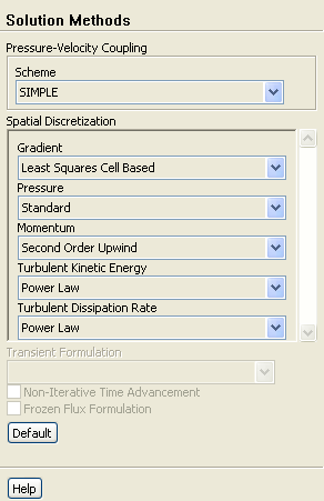
figure Solution Methods

figure

(a)   Select Second Order Upwind from the Momentum drop-down list in the Spatial Discretization group box.

(b)   Select Power Law from the Turbulent Kinetic Energy and Turbulent Dissipation Rate drop-down lists.

2.   Set the solution controls.

figure Solution Controls

figure

(a)   Enter 0.2 and 0.5 for Pressure and Momentum in the Under-Relaxation Factors group box.

(b)   Enter 0.5 for Turbulent Kinetic Energy and Turbulent Dissipation Rate.

Hint:   Scroll down in the Under-Relaxation Factors group box to locate Turbulent Kinetic Energy and Turbulent Dissipation Rate.

Note:   For this problem, it was found that these under-relaxation factors worked well.

For tips on how to adjust the under-relaxation parameters for different situations, see this section in the separate User's Guide.

3.   Enable the plotting of residuals during the calculation.

figure Monitors figure figure Residuals figure Edit...

figure

(a)   Ensure that the Plot is enabled in the Options group box.

(b)   Click OK to close the Residual Monitors dialog box.

4.   Enable the plotting of mass flow rate at the flow exit.

figure Monitors (Surface Monitors) figure Create...

figure

(a)   Retain surf-mon-1 for Name.

(b)   Enable Plot and Write.

(c)   Retain surf-mon-1.out for File Name.

(d)   Select Mass Flow Rate from the Report Type drop-down list.

(e)   Select pressure-outlet-stator from the Surfaces selection list.

(f)   Click OK to close the Surface Monitor dialog box.

5.   Initialize the flow field.

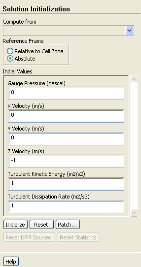
figure Solution Initialization

figure

(a)   Select Absolute in the Reference Frame list.

  For rotor-stator problems, initializing in the absolute frame is preferable, as initializing in the relative frame would introduce a non-uniform swirl velocity into the stationary domain.

(b)   Enter -1 for Z Velocity in the Initial Values group box.

(c)   Click Initialize.

6.   Save the case file ( fanstage.cas.gz).

File $\rightarrow$ Write $\rightarrow$ Case...

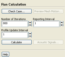
7.   Start the calculation by requesting 800 iterations.

figure Run Calculation

figure

figure   

Calculating until the mass flow rate converges will require some CPU time due to the number of iterations required. Instead of calculating the solution, you can read the data file ( fanstage.dat.gz) with the pre-calculated solution, and proceed to the postprocessing section of the tutorial (Step 9). This data file can be found in the mixing_plane/solution-files folder that was created after you unzipped the original file.

  The solution will converge after approximately 740 iterations. However, the residual history plot is only one indication of solution convergence. Note that the mass flow rate has not yet reached a constant value. To remedy this, you will reduce the convergence criterion for the continuity equation and iterate until the mass flow rate reaches a constant value.

8.   Save the case and data files ( fanstage.cas.gz and fanstage.dat.gz).

File $\rightarrow$ Write $\rightarrow$ Case & Data...

9.   Reduce the convergence criterion for the continuity equation.

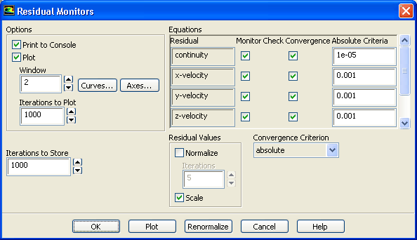
figure Monitors figure figure Residuals figure Edit...

figure

(a)   Enter 1e-05 for Absolute Criteria for continuity.

(b)   Click OK to close the Residual Monitors dialog box.

Note:   In this case, you will continue the calculation to obtain better global mass conservation; thus, only the convergence tolerance for the continuity equation is adjusted. In general, the convergence behavior of the continuity equation is a good indicator of the overall convergence of the solution.

10.   Request 1200 more iterations.

figure Run Calculation

   ANSYS FLUENT will complete the given number of iterations. After a total of about 1400 iterations the mass flow rate has leveled off and hence, we can consider that the solution is converged. The mass flow rate history is shown in Figure  11.3.

Figure 11.3: Mass Flow Rate History
figure

11.   Save the case and data files ( fanstage1.cas.gz and fanstage1.dat.gz).

File $\rightarrow$ Write $\rightarrow$ Case & Data...

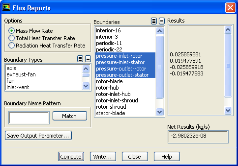
12.   Check the mass flux balance.

figure Reports figure figure Fluxes figure Set Up...

figure   

Although the mass flow rate history indicates that the solution is converged, you should also check the mass fluxes through the domain to ensure that mass is being conserved.

figure

(a)   Retain the default selection of Mass Flow Rate in the Options list.

(b)   Select pressure-inlet-rotor, pressure-inlet-stator, pressure-outlet-rotor, and pressure-outlet-stator from the Boundaries selection list.

(c)   Click Compute and close the Flux Reports dialog box.

figure   

The net mass imbalance should be a small fraction (say, 0.5%) of the total flux through the system. If a significant imbalance occurs, you should decrease your residual tolerances by at least an order of magnitude and continue iterating.

Note:   The fluxes for the portions of the rotor and stator that have been modeled are different. However, the flux for the whole rotor and the whole stator are very nearly equal: approximately 0.23265 kg/s (0.02585 $\times$ 9 rotor blades), versus approximately 0.23364 kg/s (0.01947 $\times$ 12 stator blades).


next up previous contents Previous: Step 7: Boundary Conditions
Up: Using the Mixing Plane
Next: Step 9: Postprocessing
Release 12.0 © ANSYS, Inc. 2009-02-09