Step 9: Postprocessing

1.   Create an isosurface at $y=0.12$ m.

Surface $\rightarrow$ Iso-Surface...

  The surface $y=0.12$ m is a midspan slice through the mesh. This view is good for looking at the blade-to-blade flow field.

(a)    Select Mesh... and Y-Coordinate from the Surface of Constant drop-down lists.

(b)   Click Compute to update the minimum and maximum values.

(c)   Enter 0.12 for Iso-Values.

(d)   Enter y=0.12 for New Surface Name.

(e)   Click Create to create the isosurface.

2.   Create an isosurface at $z=-0.1$ m.

Surface $\rightarrow$ Iso-Surface...

  The surface $z=-0.1$ m is an axial plane downstream of the stator. This will be used to plot circumferentially-averaged profiles.

(a)   Select Mesh... and Z-Coordinate from the Surface of Constant drop-down lists.

(b)   Click Compute to update the minimum and maximum values.

(c)   Enter -0.1 for Iso-Values.

(d)   Enter z=-0.1 for New Surface Name.

Note:   The default name that ANSYS FLUENT displays in the New Surface Name field (i.e., z-coordinate-17) indicates that this is surface number 17. This fact will be used later in the tutorial when you plot circumferential averages.

(e)   Click Create to create the isosurface.

(f)   Close the Iso-Surface dialog box.

3.   Display velocity vectors on the midspan surface $y=0.12$ (Figure  11.4).

Graphics and Animations Vectors Set Up...

(a)   Retain the default selection of arrow from the Style drop-down list.

(b)   Enter 10 for Scale.

(c)   Set Skip to 2.

(d)   Select y=0.12 from the Surfaces selection list.

(e)   Click Display to plot the velocity vectors.

(f)   Rotate and zoom the view to get the display shown in Figure  11.4.

Figure 11.4: Velocity Vectors on $y=0.12$ Near the Stator Blade

  Plotting the velocity field in this manner gives a good indication of the midspan flow over the stator. For the rotor, it is instructive to similarly plot the relative velocity field.

(g)   Close the Vectors dialog box.

4.   Plot a circumferential average of the total pressure on the plane $z=-0.1$.

(a)   Type the text commands in the console, as shown in green in the following dialog:

> plot

/plot> circum-avg-radial

averages of> total-pressure

on surface [] 17

number of bands [5] 15

Note:   Surface 17 is the surface $z=-0.1$ you created earlier. For increased resolution, 15 bands are used instead of the default 5.

(b)   Enter the name of the output file as circum-plot.xy when prompted.

Computing r-coordinate ...
Clipping to r-coordinate ... done.
Computing "total-pressure" ...
Computing averages ... done.
Creating radial-bands surface (32 31 30 29 28 27 26 25 24 23 22 21 20 19 18).
filename [""] "circum-plot.xy"
order points? [no]

(c)   Retain the default of no when asked to order points.

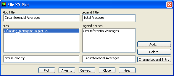
(d)   Display the circumferential average.

Plots File Set Up...

i.   Click Add... and select the file circum-plot.xy in the Select File dialog box.

ii.   Click Plot and close the File XY Plot dialog box.

  The radial variation in the total pressure can be seen to be very non-uniform in this plot (Figure  11.5). This implies that losses are largest near the hub.

Figure 11.5: Plot of Circumferential Average of the Total Pressure on the Plane $z=-0.1$.

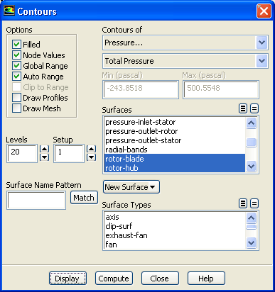
5.   Display filled contours of total pressure.

Graphics and Animations Contours Set Up...

(a)   Enable Filled in the Options group box.

(b)   Select Pressure... and Total Pressure from the Contours of drop-down lists.

(c)   Select rotor-blade and rotor-hub from the Surfaces selection list.

(d)   Click Display and close the Contours dialog box.

(e)   Rotate the view to get the display as shown in Figure  11.6.

  The pressure contours are displayed in Figure  11.6. Notice the high pressure that occurs on the leading edge of the rotor blade due to the motion of the blade.

Figure 11.6: Contours of Total Pressure for the Rotor Blade and Hub

6.   Display the total pressure profiles at the outlet of the rotor.

Plots Profile Data Set Up...

(a)   Select pressure-outlet-rotor from the Profile selection list.

(b)   Select p0 from the Y Axis Function selection list.

(c)   Click Plot and close the Plot Profile Data dialog box.

Figure 11.7: Profile Plot of Total Pressure for the Rotor

Note:   The profiles shown are area-averaged profiles computed by the mixing plane model.