Step 7: Solution Using the Standard $k$- $\epsilon$ Model

1.   Set the solution parameters.

Solution Methods

(a)   Retain the default selection of Least Squares Cell Based from the Gradient list in the Spatial Discretization group box.

(b)   Select PRESTO! from the Pressure drop-down list in the Spatial Discretization group box.

  The PRESTO! scheme is well suited for steep pressure gradients involved in rotating flows. It provides improved pressure interpolation in situations where large body forces or strong pressure variations are present as in swirling flows.

(c)   Select Second Order Upwind from the Momentum, Swirl Velocity, Turbulent Kinetic Energy, and Turbulent Dissipation Rate drop-down lists.

  Use the scroll bar to access the discretization schemes that are not initially visible in the task page.

2.   Set the solution controls.

Solution Controls

(a)   Retain the default values in the Under-Relaxation Factors group box.

Note:   For this problem, the default under-relaxation factors are satisfactory. However, if the solution diverges or the residuals display large oscillations, you may need to reduce the under-relaxation factors from their default values.

For tips on how to adjust the under-relaxation parameters for different situations, see this section in the separate User's Guide.

3.   Enable the plotting of residuals during the calculation.

Monitors Residuals Edit...

(a)   Ensure that Plot is enabled in the Options group box.

(b)   Click OK to close the Residual Monitors dialog box.

Note:   For this calculation, the convergence tolerance on the continuity equation is kept at 0.001. Depending on the behavior of the solution, you can reduce this value if necessary.

4.   Enable the plotting of mass flow rate at the flow exit.

Monitors ( Surface Monitors) Create...

(a)   Enable the Plot and Write options for surf-mon-1.

Note:   When the Write option is selected in the Surface Monitor dialog box,the mass flow rate history will be written to a file. If you do not enable the Write option, the history information will be lost when you exit ANSYS FLUENT.

(b)   Select Mass Flow Rate from the Report Type drop-down list.

(c)   Select pressure-outlet-3 from the Surfaces selection list.

(d)   Click OK in the Surface Monitor dialog box to enable the monitor.

5.   Initialize the flow field using the boundary conditions set at velocity-inlet-2.

Solution Initialization

(a)   Select velocity-inlet-2 from the Compute From drop-down list.

(b)   Click Initialize.

6.   Save the case file ( disk-ke.cas.gz).

File $\rightarrow$ Write $\rightarrow$ Case...

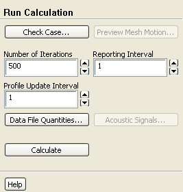
7.   Start the calculation by requesting 500 iterations.

Run Calculation

(a)   Enter 500 for the Number of Iterations.

(b)   Click Calculate.

  Throughout the calculation, ANSYS FLUENT will report reversed flow at the exit. This is reasonable for the current case. The solution should be sufficiently converged after approximately 225 iterations. The mass flow rate history is shown in Figure  9.3.

Figure 9.3: Mass Flow Rate History ( $k$- $\epsilon$ Turbulence Model)

8.   Check the mass flux balance.

Reports Fluxes Set Up...

Although the mass flow rate history indicates that the solution is converged, you should also check the net mass fluxes through the domain to ensure that mass is being conserved.

(a)   Select velocity-inlet-2 and pressure-outlet-3 from the Boundaries selection list.

(b)   Retain the default Mass Flow Rate option.

(c)   Click Compute and close the Flux Reports dialog box.

The net mass imbalance should be a small fraction (say, 0.5%) of the total flux through the system. If a significant imbalance occurs, you should decrease the residual tolerances by at least an order of magnitude and continue iterating.

9.   Save the data file ( disk-ke.dat.gz).

File $\rightarrow$ Write $\rightarrow$ Data...

Note:   If you choose a file name that already exists in the current folder, ANSYS FLUENT will prompt you for confirmation to overwrite the file.