Step 8: Postprocessing for the Standard $k$- $\epsilon$ Solution

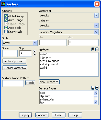
1.   Display the velocity vectors.

Graphics and Animations Vectors Set Up...

(a)   Enter 50 for Scale

(b)   Set Skip to 1.

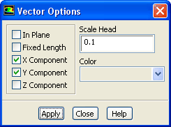
(c)   Click the Vector Options... button to open the Vector Options dialog box.

i.   Disable Z Component.

  This allows you to examine only the non-swirling components.

ii.   Click Apply and close the Vector Options dialog box.

(d)   Click Display in the Vectors dialog box to plot the velocity vectors.

  A magnified view of the velocity field displaying a counter-clockwise circulation of the flow is shown in Figure  9.4.

Figure 9.4: Magnified View of Velocity Vectors within the Disk Cavity

(e)   Close the Vectors dialog box.

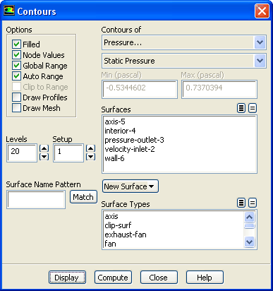
2.   Display filled contours of static pressure.

Graphics and Animations Contours Set Up...

(a)   Enable Filled in the Options group box.

(b)   Retain the selection of Pressure... and Static Pressure from the Contours of drop-down lists.

(c)   Click Display and close the Contours dialog box.

  The pressure contours are displayed in Figure  9.5. Notice the high pressure that occurs on the right disk near the hub due to the stagnation of the flow entering from the bore.

Figure 9.5: Contours of Static Pressure for the Entire Disk Cavity

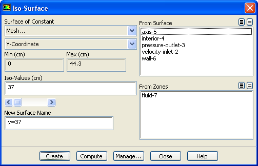
3.   Create a constant $y$-coordinate line for postprocessing.

Surface $\rightarrow$ Iso-Surface...

(a)   Select Mesh... and Y-Coordinate from the Surface of Constant drop-down lists.

(b)   Click Compute to update the minimum and maximum values.

(c)   Enter 37 in the Iso-Values field.

  This is the radial position along which you will plot the radial velocity profile.

(d)   Enter y=37cm for the New Surface Name.

(e)   Click Create to create the isosurface.

Note:   The name you use for an isosurface can be any continuous string of characters (without spaces).

(f)   Close the Iso-Surface dialog box.

4.   Plot the radial velocity distribution on the surface y=37cm.

Plots XY Plot Set Up...

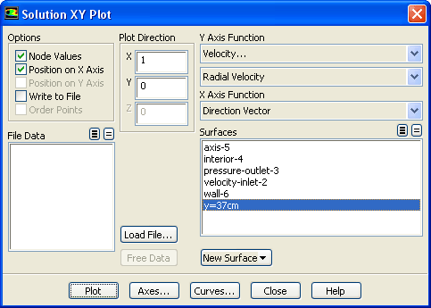
(a)   Select Velocity... and Radial Velocity from the Y Axis Function drop-down lists.

(b)   Select the y-coordinate line y=37cm from the Surfaces selection list.

(c)   Click Plot.

   Figure  9.6 shows a plot of the radial velocity distribution along $y=37$ $cm$.

Figure 9.6: Radial Velocity Distribution--Standard $k$- $\epsilon$ Solution

(d)   Enable Write to File in the Options group box to save the radial velocity profile.

(e)   Click the Write... button to open the Select File dialog box.

i.   Enter ke-data.xy in the XY File text entry box and click OK.

5.   Plot the wall y+ distribution on the rotating disk wall along the radial direction (Figure  9.7).

Plots XY Plot Set Up...

(a)   Disable Write to File in the Options group box.

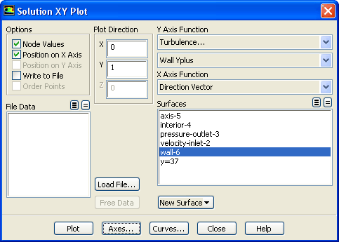
(b)   Select Turbulence... and Wall Yplus from the Y Axis Function drop-down lists.

(c)   Deselect y=37cm and select wall-6 from the Surfaces selection list.

(d)   Enter 0 and 1 for X and Y respectively in the Plot Direction group box.

(e)   Click the Axes... button to open the Axes - Solution XY Plot dialog box.

i.   Retain the default selection of X from the Axis group box.

ii.   Disable Auto Range in the Options group box.

iii.   Retain the default value of 0 for Minimum and enter 43 for Maximum in the Range group box.

iv.   Click Apply and close the Axes - Solution XY Plot dialog box.

(f)   Click Plot in the Solution XY Plot dialog box.

  Figure  9.7 shows a plot of wall y+ distribution along wall-6.

Figure 9.7: Wall Yplus Distribution on wall-6--Standard $k$- $\epsilon$ Solution

(g)   Enable Write to File in the Options group box to save the wall y+ profile.

(h)   Click the Write... button to open the Select File dialog box.

i.   Enter ke-yplus.xy in the XY File text entry box and click OK.

Note:   Ideally, while using enhanced wall treatment, the wall y+ should be in the order of 1 (at least $<$ 5) to resolve viscous sublayer. The plot justifies the applicability of enhanced wall treatment to the given mesh.

(i)   Close the Solution XY Plot dialog box.