Step 7: Solution

1.   Set the solution parameters.

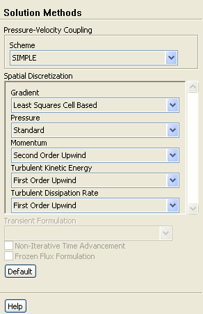
Solution Methods

(a)   Retain the default selection of Least Squares Cell Based from the Gradient drop-down list in the Spatial Discretization group box.

(b)   Select Second Order Upwind from the Momentum drop-down list.

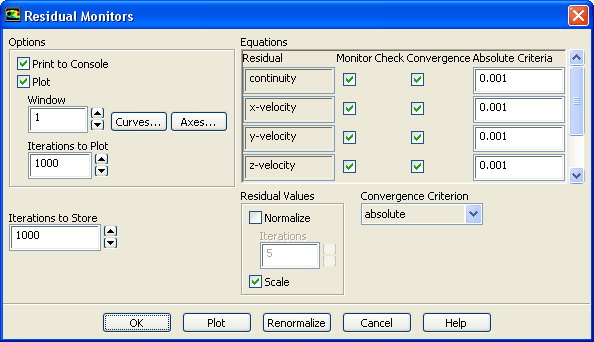
2.   Enable the plotting of residuals during the calculation.

Monitors Residuals Edit...

(a)   Retain the default settings.

(b)   Click OK to close the Residual Monitors dialog box.

3.   Enable the plotting of the mass flow rate at the outlet.

Monitors (Surface Monitors) Create...

(a)   Enable Plot and Write.

(b)   Select Mass Flow Rate from the Report Type drop-down list.

(c)   Select outlet in the Surfaces selection list.

(d)   Click OK to close the Surface Monitor dialog box.

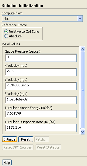
4.   Initialize the solution from the inlet.

Solution Initialization

(a)   Select inlet from the Compute From drop-down list.

(b)   Click Initialize.

5.   Save the case file ( catalytic_converter.cas).

File $\rightarrow$ Write $\rightarrow$ Case...

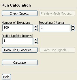
6.   Run the calculation by requesting 100 iterations.

Run Calculation

(a)   Enter 100 for Number of Iterations.

(b)   Click Calculate to begin the iterations.

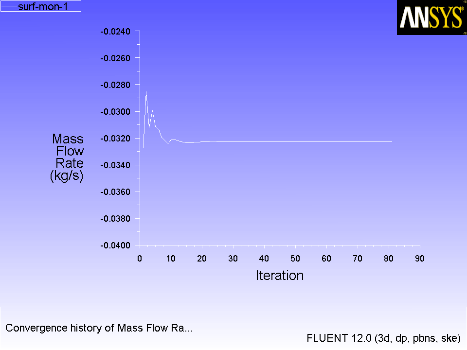
  The ANSYS FLUENT calculation will converge in approximately 80 iterations. The mass flow rate monitor flattens out, as seen in Figure  8.3.

Figure 8.3: Surface Monitor Plot of Mass Flow Rate with Number of Iterations

7.   Save the case and data files ( catalytic_converter.cas and
catalytic_converter.dat).

File $\rightarrow$ Write $\rightarrow$ Case & Data...

Note:   If you choose a file name that already exists in the current folder, ANSYS FLUENT will prompt you for confirmation to overwrite the file.