Step 8: Postprocessing

1.   Create a surface passing through the centerline for postprocessing purposes.

Surface $\rightarrow$ Iso-Surface...

(a)   Select Mesh... and Y-Coordinate from the Surface of Constant drop-down lists.

(b)   Click Compute to calculate the Min and Max values.

(c)   Retain the default value of 0 for Iso-Values.

(d)   Enter y=0 for New Surface Name.

(e)   Click Create.

Note:   To interactively place the surface on your mesh, use the slider bar in the Iso-Surface dialog box.

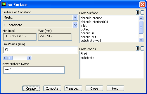
2.   Create cross-sectional surfaces at locations on either side of the substrate, as well as at its center.

Surface $\rightarrow$ Iso-Surface...

(a)   Select Mesh... and X-Coordinate from the Surface of Constant drop-down lists.

(b)   Click Compute to calculate the Min and Max values.

(c)   Enter 95 for Iso-Values.

(d)   Enter x=95 for the New Surface Name.

(e)   Click Create.

(f)   In a similar manner, create surfaces named x=130 and x=165 with Iso-Values of 130 and 165, respectively.

(g)   Close the Iso-Surface dialog box after all the surfaces have been created.

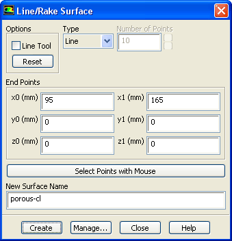
3.   Create a line surface for the centerline of the porous media.

Surface $\rightarrow$ Line/Rake...

(a)   Enter the coordinates of the end points of the line in the End Points group box as shown.

(b)   Enter porous-cl for the New Surface Name.

(c)   Click Create to create the surface.

(d)   Close the Line/Rake Surface dialog box.

4.   Display the two wall zones ( substrate-wall and wall).

Graphics and Animations Mesh Set Up...

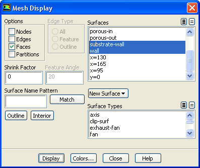
(a)   Disable Edges and enable Faces in the Options group box.

(b)   Deselect inlet and outlet in the Surfaces selection list, and make sure that only substrate-wall and wall are selected.

(c)   Click Display and close the Mesh Display dialog box.

(d)   Rotate the view and zoom so that the display is similar to Figure  8.2.

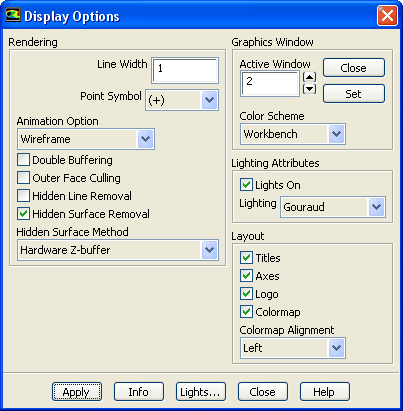
5.   Set the lighting for the display.

Graphics and Animations Options...

(a)   Enable Lights On in the Lighting Attributes group box.

(b)   Select Gouraud from the Lighting drop-down list.

(c)   Click Apply and close the Display Options dialog box.

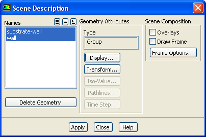
6.   Set the transparency parameter for the wall zones ( substrate-wall and wall).

Graphics and Animations Scene...

(a)   Select substrate-wall and wall in the Names selection list.

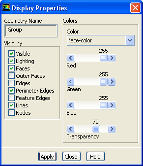
(b)   Click the Display... button in the Geometry Attributes group box to open the Display Properties dialog box.

i.   Make sure that Red, Green, and Blue sliders are set to the maximum position (i.e. 255).

ii.   Set the Transparency slider to 70.

iii.   Click Apply and close the Display Properties dialog box.

(c)   Click Apply and close the Scene Description dialog box.

7.   Display velocity vectors on the y=0 surface (Figure  8.4).

Graphics and Animations Vectors Set Up...

(a)   Enable Draw Mesh in the Options group box to open the Mesh Display dialog box.

i.   Make sure that substrate-wall and wall are selected in the Surfaces selection list.

ii.   Click Display and close the Mesh Display dialog box.

(b)   Enter 5 for Scale.

(c)   Set Skip to 1.

(d)   Select y=0 in the Surfaces selection list.

(e)   Click Display and close the Vectors dialog box.

Figure 8.4: Velocity Vectors on the y=0 Plane

  The flow pattern shows that the flow enters the catalytic converter as a jet, with recirculation on either side of the jet. As it passes through the porous substrate, it decelerates and straightens out, and exhibits a more uniform velocity distribution. This allows the metal catalyst present in the substrate to be more effective.

8.   Display filled contours of static pressure on the y=0 plane (Figure  8.5).

Graphics and Animations Contours Set Up...

(a)   Enable Filled in the Options group box.

(b)   Enable Draw Mesh to open the Mesh Display dialog box.

i.   Make sure that substrate-wall and wall are selected in the Surfaces selection list.

ii.   Click Display and close the Mesh Display dialog box.

(c)   Make sure that Pressure... and Static Pressure are selected from the Contours of drop-down lists.

(d)   Select y=0 in the Surfaces selection list.

(e)   Click Display and close the Contours dialog box.

  The pressure changes rapidly in the middle section, where the fluid velocity changes as it passes through the porous substrate. The pressure drop can be high, due to the inertial and viscous resistance of the porous media. Determining this pressure drop is one of the goals of the CFD analysis. In the next step, you will learn how to plot the pressure drop along the centerline of the substrate.

Figure 8.5: Contours of Static Pressure on the y=0 plane

9.   Plot the static pressure across the line surface porous-cl (Figure  8.6).

Plots XY Plot Set Up...

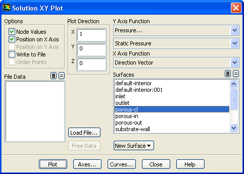
(a)   Make sure that Pressure... and Static Pressure are selected from the Y Axis Function drop-down lists.

(b)   Select porous-cl in the Surfaces selection list.

(c)   Click Plot and close the Solution XY Plot dialog box.

Figure 8.6: Plot of Static Pressure on the porous-cl Line Surface

  As seen in Figure  8.6, the pressure drop across the porous substrate is approximately 300 Pa.

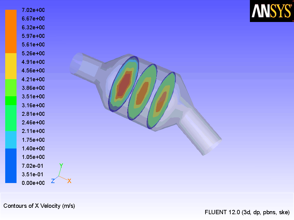
10.   Display filled contours of the velocity in the X direction on the x=95, x=130, and x=165 surfaces (Figure  8.7).

Graphics and Animations Contours Set Up...

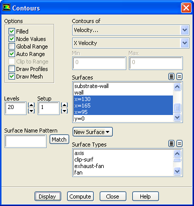
(a)   Enable Filled in the Options group box.

(b)   Enable Draw Mesh to open the Mesh Display dialog box.

i.   Make sure that substrate-wall and wall are selected in the Surfaces selection list.

ii.   Click Display and close the Mesh Display dialog box.

(c)   Disable Global Range in the Options group box.

(d)   Select Velocity... and X Velocity from the Contours of drop-down lists.

(e)   Select x=130, x=165, and x=95 in the Surfaces selection list.

(f)   Click Display and close the Contours dialog box.

Figure 8.7: Contours of the X Velocity on the x=95, x=130, and x=165 Surfaces

  The velocity profile becomes more uniform as the fluid passes through the porous media. The velocity is very high at the center (the area in red) just before the nitrogen enters the substrate and then decreases as it passes through and exits the substrate. The area in green, which corresponds to a moderate velocity, increases in extent.

11.   Use numerical reports to determine the average, minimum, and maximum of the velocity distribution before and after the porous substrate.

Reports Surface Integrals Set Up...

(a)   Select Mass-Weighted Average from the Report Type drop-down list.

(b)   Select Velocity and X Velocity from the Field Variable drop-down lists.

(c)   Select x=165 and x=95 in the Surfaces selection list.

(d)   Click Compute.

(e)   Select Facet Minimum from the Report Type drop-down list and click Compute.

(f)   Select Facet Maximum from the Report Type drop-down list and click Compute.

  The numerical report of average, maximum and minimum velocity can be seen in the main ANSYS FLUENT console.

(g)   Close the Surface Integrals dialog box.

  The spread between the average, maximum, and minimum values for X velocity gives the degree to which the velocity distribution is non-uniform. You can also use these numbers to calculate the velocity ratio (i.e., the maximum velocity divided by the mean velocity) and the space velocity (i.e., the product of the mean velocity and the substrate length).

Custom field functions and UDFs can be also used to calculate more complex measures of non-uniformity, such as the standard deviation and the gamma uniformity index.

 Mass-Weighted Average
                      X Velocity                (m/s)
-------------------------------- --------------------
                           x=165            4.0038509
                            x=95            5.2266927
                ---------------- --------------------
                             Net            4.6102977

         Minimum of Facet Values
                      X Velocity                (m/s)
-------------------------------- --------------------
                           x=165            2.4261272
                            x=95           0.31741163
                ---------------- --------------------
                             Net           0.31741163

         Maximum of Facet Values
                      X Velocity                (m/s)
-------------------------------- --------------------
                           x=165            6.1665144
                            x=95            7.7021732
                ---------------- --------------------
                             Net            7.7021732