Step 4: Setting Up the CFD Simulation in ANSYS FLUENT

Now that you have created a computational mesh for the elbow geometry, you can proceed to setting up a CFD analysis using ANSYS FLUENT.

1.   Start ANSYS FLUENT.

In the ANSYS Workbench Project Schematic, double-click the Setup cell in the elbow fluid flow analysis system. You can also right-click on the Setup cell to display the context menu where you can select the Edit option.

When ANSYS FLUENT is first started, FLUENT Launcher is displayed, allowing you to view and/or set certain ANSYS FLUENT start-up options.

   ANSYS FLUENT Launcher allows you to decide which version of ANSYS FLUENT you will use, based on your geometry and on your processing capabilities.

Figure 1.16: ANSYS FLUENT Launcher

(a)   Ensure that the proper options are enabled.

Note that the Dimension setting is already filled in and cannot be changed, since ANSYS FLUENT automatically sets it based on the mesh or geometry for the current system.

i.   Make sure that Serial from the Processing Options list is enabled.

ii.   Make sure that the Display Mesh After Reading, Embed Graphics Windows, and Workbench Color Scheme options are enabled.

Note:   An option is enabled when there is a check mark in the check box, and disabled when the check box is empty. To change an option from disabled to enabled (or vice versa), click the check box or the text.

iii.   Make sure that the Double-Precision option is disabled.

(b)   Click OK to launch ANSYS FLUENT.

Figure 1.17: The ANSYS FLUENT Application

Note:   The mesh is automatically loaded and displayed in the graphics window by default.

2.   Set some general settings for the CFD analysis.

  Select General in the navigation pane to perform the mesh-related activities and to choose a solver.

General

(a)   Change the units for length.

Since we want to specify and view values based on a unit of length in inches from within ANSYS FLUENT, change the units of length within ANSYS FLUENT from meters (the default) to inches.

Note that the ANSYS Meshing application automatically converts and exports meshes for ANSYS FLUENT using meters (m) as the unit of length regardless of what units were used to create them. This is so you do not have to scale the mesh in ANSYS FLUENT under ANSYS Workbench.

General Units...

This displays the Set Units dialog box.

i.   Select length in the Quantities list.

ii.   Select in in the Units list.

iii.   Close the dialog box.

   Now, all subsequent inputs that require a value based on a unit of length can be specified in inches rather than meters.

(b)   Check the mesh.

General Check

   ANSYS FLUENT will report the results of the mesh check in the console.

 Domain Extents:
   x-coordinate: min (m) = -2.032000e-001, max (m) = 2.032000e-001
   y-coordinate: min (m) = -2.286000e-001, max (m) = 2.032000e-001
   z-coordinate: min (m) = -2.332875e-018, max (m) = 5.079992e-002
 Volume statistics:
   minimum volume (m3): 1.106292e-009
   maximum volume (m3): 1.406825e-006
     total volume (m3): 2.607593e-003
 Face area statistics:
   minimum face area (m2): 1.042914e-006
   maximum face area (m2): 2.850931e-004
 Checking number of nodes per cell.
 Checking number of faces per cell.
 Checking thread pointers.
 Checking number of cells per face.
 Checking face cells.
 Checking cell connectivity.
 Checking bridge faces.
 Checking right-handed cells.
 Checking face handedness.
 Checking face node order.
 Checking closed cells.
 Checking contact points.
 Checking element type consistency.
 Checking boundary types:
 Checking face pairs.
 Checking wall distance.
 Checking node count.
 Checking nosolve cell count.
 Checking nosolve face count.
 Checking face children.
 Checking cell children.
 Checking storage.
Done.

Note:   The minimum and maximum values may vary slightly when running on different platforms. The mesh check will list the minimum and maximum $x$ and $y$ values from the mesh in the default SI unit of meters. It will also report a number of other mesh features that are checked. Any errors in the mesh will be reported at this time. Ensure that the minimum volume is not negative, since ANSYS FLUENT cannot begin a calculation when this is the case.

3.   Set up your models for the CFD simulation.

Models

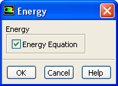
(a)   Enable heat transfer by activating the energy equation.

Models Energy Edit...

   You can also double-click a list item in order to open the corresponding dialog box.

i.   Enable the Energy Equation option.

ii.   Click OK to close the Energy dialog box.

(b)   Enable the $k$- $\epsilon$ turbulence model.

Models Viscous Edit...

i.   Select k-epsilon from the Model list.

   The Viscous Model dialog box will expand.

ii.   Select Realizable from the k-epsilon Model list.

iii.   Click OK to accept the model and close the Viscous Model dialog box.

4.   Set up your materials for the CFD simulation.

Materials

(a)   Create a new material called water using the Create/Edit Materialsdialog box (Figure  1.18).

Materials Fluid Create/Edit...

i.   Enter water for Name.

ii.   Enter the following values in the Properties group box:

Property	Value
Density	1000 ${\rm kg/m}^3$
$c_p$	4216 ${\rm J/kg-K}$
Thermal Conductivity	0.677 ${\rm W/m-K}$
Viscosity	8e-04 ${\rm kg/m-s}$

Figure 1.18: The Create/Edit Materials Dialog Box

iii.   Click Change/Create.

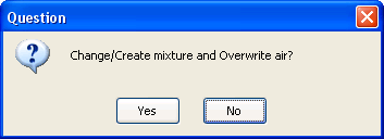
  A Question dialog box will open, asking if you want to overwrite air. Click No so that the new material water is added to the list of materials which originally contained only air.

Extra:   You could have copied the material water-liquid (h2o $<$l $>$) from the materials database (accessed by clicking the FLUENT Database... button). If the properties in the database are different from those you wish to use, you can edit the values in the Properties group box in the Create/Edit Materials dialog box and click Change/Create to update your local copy. The original copy will not be affected.

iv.   Make sure that there are now two materials (water and air) defined locally by examining the Fluent Fluid Materials drop-down list.

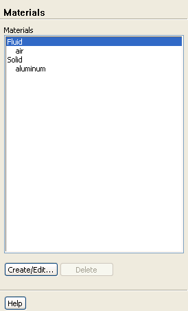
  Both the materials will also be listed under Fluid in the Materials task page.

v.   Close the Create/Edit Materials dialog box.

5.   Set up the cell zone conditions for the CFD simulation.

Cell Zone Conditions

(a)   Set the cell zone conditions for the fluid zone.

i.   Select fluid in the Zones list in the Cell Zone Conditions task page, then click the Edit... button to open the Fluid dialog box.

   You can also double-click a list item in order to open the corresponding dialog box.

ii.   In the Fluid dialog box, select water from the Material Name drop-down list.

iii.   Click OK to close the Fluid dialog box.

6.   Set up the boundary conditions for the CFD analysis.

Boundary Conditions

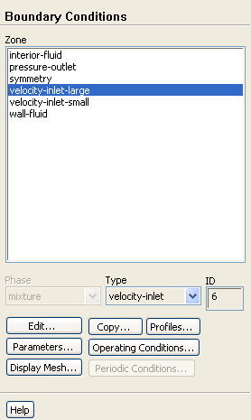
(a)   Set the boundary conditions at the cold inlet ( velocity-inlet-large).

Boundary Conditions velocity-inlet-large Edit...

Hint:   If you are unsure of which inlet zone corresponds to the cold inlet, you can probe the mesh display using the right mouse button or the probe toolbar button ( ) as described in a previous step. The information will be displayed in the ANSYS FLUENT console, and the zone you probed will be automatically selected from the Zone selection list in the Boundary Conditions task page.

i.   Select Components from the Velocity Specification Method drop-down list.

  The Velocity Inlet dialog box will expand.

ii.   Enter 0.4  ${\rm m/s}$ for X-Velocity.

iii.   Retain the default value of 0  ${\rm m/s}$ for both Y-Velocity and Z-Velocity.

iv.   Select Intensity and Hydraulic Diameter from the Specification Method drop-down list in the Turbulence group box.

v.   Enter 5 ${\rm\%}$ for Turbulent Intensity.

vi.   Enter 4 in for Hydraulic Diameter.

  The hydraulic diameter $D_h$ is defined as:

where $A$ is the cross-sectional area and $P_w$ is the wetted perimeter.

vii.   Click the Thermal tab.

viii.   Enter 293.15  ${\rm K}$ for Temperature.

ix.   Click OK to close the Velocity Inlet dialog box.

(b)   In a similar manner, set the boundary conditions at the hot inlet ( velocity-inlet-small), using the values in the following table:

Boundary Conditions velocity-inlet-small Edit...

Velocity Specification Method	Components
X-Velocity	0  ${\rm m/s}$
Y-Velocity	1.2  ${\rm m/s}$
Z-Velocity	0  ${\rm m/s}$
Specification Method	Intensity & Hydraulic Diameter
Turbulent Intensity	5 ${\rm\%}$
Hydraulic Diameter	1 in
Temperature	313.15  ${\rm K}$

(c)   Set the boundary conditions at the outlet ( pressure-outlet), as shown in the Pressure Outlet dialog box.

Boundary Conditions pressure-outlet Edit...

Note:    ANSYS FLUENT will use the backflow conditions only if the fluid is flowing into the computational domain through the outlet. Since backflow might occur at some point during the solution procedure, you should set reasonable backflow conditions to prevent convergence from being adversely affected.

7.   Set up solution parameters for the CFD simulation.

  In the steps that follow, you will set up and run the calculation using the task pages listed under the Solution heading in the navigation pane.

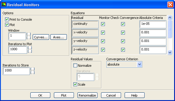
(a)   Change the convergence criteria for the continuity equation residual.

Monitors Residuals Edit...

i.   Make sure that Plot is enabled in the Options group box.

ii.   Enter 1e-05 for the Absolute Criteria of continuity, as shown in the Residual Monitor dialog box.

iii.   Click OK to close the Residual Monitors dialog box.

Note:   By default, all variables will be monitored and checked by ANSYS FLUENT as a means to determine the convergence of the solution.

(b)   Initialize the flow field, using the boundary conditions settings at the cold inlet ( velocity-inlet-large) as a starting point.

Solution Initialization

i.   Select velocity-inlet-large from the Compute From drop-down list.

ii.   Enter 1.2  ${\rm m/s}$ for Y Velocity in the Initial Values group box.

Note:   While an initial X Velocity is an appropriate guess for the horizontal section, the addition of a Y Velocity component will give rise to a better initial guess throughout the entire elbow.

iii.   Click Initialize.

(c)   Check to see if the case conforms to best practices.

Run Calculation Check Case

i.   Click the Solver tab and examine the Recommendation in the Manual Implementation group box.

   The only recommendation for this mesh is to use discretization of a higher order. This recommendation can be ignored for the time being, as it was performed in the first tutorial in the separate Tutorial Guide.

ii.   Close the Case Check dialog box.

Note that, while you are working in the ANSYS FLUENT application, the states of the Setup and Solution cells in the fluid flow FLUENT analysis system in ANSYS Workbench are changing. For example: The state of the Setup cell becomes Up-to-Date and the state of the Solution cell becomes Refresh Required after the Solution Initialization task page is visited and the number of iterations is specified. The state of the Solution cell is Update Required while iterations are taking place. The state of the Solution cell is Up-to-Date when the specified number of iterations are complete (or if convergence is reached). For more information, see the separate FLUENT in Workbench User's Guide.

8.   Calculate a solution.

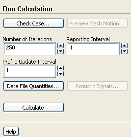
(a)   Start the calculation by requesting 250 iterations.

Run Calculation

i.   Enter 250 for Number of Iterations.

ii.   Click Calculate.

Note that ANSYS FLUENT settings file is written before the calculation begins. For more information about settings files, see the separate FLUENT in Workbench User's Guide.

  As the calculation progresses, the residuals will be plotted in the graphics window (Figure  1.19).

Figure 1.19: Residuals for the Converged Solution

Note:   The solution will be stopped by ANSYS FLUENT after approximately 230 iterations, when the residuals reach their specified values. The exact number of iterations will vary, depending on the platform being used. An Information dialog box will open to alert you that the calculation is complete. Click OK in the Information dialog box to proceed.

Since the residual values vary slightly by platform, the plot that appears on your screen may not be exactly the same as the one shown here.

9.   View the files generated by ANSYS Workbench.

View $\rightarrow$ Files

Figure 1.20: ANSYS Workbench Displaying the Files View for the Project After Generating a Solution

Note the addition of the ANSYS FLUENT settings file ( FFF.set) to the list of files. Also note that the status of the Solution cell is now up-to-date.