23.7.1 Displaying of Trajectories

When you have defined discrete phase particle injections, as described in Section  23.3, you can display the trajectories of these discrete particles using the Particle Tracks dialog box (Figure  23.7.1).

Graphics and Animations Particle Tracks Set Up...

Figure 23.7.1: The Particle Tracks Dialog Box

The procedure for drawing trajectories for particle injections is as follows:

1.   Select the particle injection(s) you wish to track in the Release from Injections list. (You can choose to track a specific particle, instead, as described below.)

2.   Set the length scale and the maximum number of steps in the Discrete Phase Model dialog box, as described in Section  23.2.8.

Models Discrete Phase Edit...

If stochastic and/or cloud tracking is desired, set the related parameters in the Set Injection Properties dialog box, as described in Section  23.3.16.

3.   Set any of the display options described below.

4.   Click the Display button to draw the trajectories or click the Pulse button to animate the particle positions. The Pulse button will become the Stop ! button during the animation, and you must click Stop ! to stop the pulsing.

For unsteady particle tracking simulations, clicking Display will show only the current location of the particles. Typically, you should select point in the Style drop-down list when displaying transient particle locations since individual positions will be displayed. The Pulse button option is not available for unsteady tracking.

Specifying Individual Particles for Display

It is also possible to display the trajectory for an individual particle stream instead of for all the streams in a given injection. To do so, you will first need to determine which particle is of interest. Use the Injections dialog box to list the particle streams in the desired injection, as described in Section  23.3.14.

Define $\rightarrow$ Injections...

Note the ID numbers listed in the first column of the listing printed in the ANSYS FLUENT console. Then perform the following steps after step 1 above:

1.   Enable the Track Single Particle Stream option in the Particle Tracks dialog box.

2.   In the Stream ID field, specify the ID number of the particle stream for which you want to plot the trajectory.

Importing Particle Data

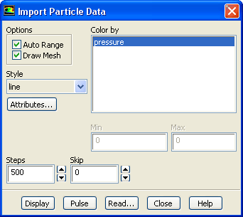
Use the Import Particle Data dialog box (Figure  23.7.2) to import particle data to display in the graphics window.

Display $\rightarrow$ Import Particle Data...

Figure 23.7.2: The Import Particle Data Dialog Box

1.   Click Read... to display a file selection dialog box where you can enter a file name and a directory that contains the imported data.

2.   Choose from the available import options by selecting Auto Range and/or Draw Mesh under Options. If you prefer to restrict the range of the scalar field, disable the Auto Range option and set the Min and Max values manually beneath the Color by list.

3.   Choose to color the particle pathlines by any of the scalar fields in the Color by list.

4.   Select a pathline style under Style. To set pathline style attributes, click the Style Attributes... button. For more information about the pathline style types, see Section  29.1.4.

5.   The value of Steps sets the maximum number of steps a particle can advance. A particle will stop when it has traveled this number of steps or when it leaves the domain.

6.   If your pathline plot is difficult to understand because there are too many paths displayed, you can "thin out'' the pathlines by changing the Skip value.

7.   Click the Display button to draw the pathlines, or click the Pulse button to animate the particle positions. The Pulse button will become the Stop ! button during the animation, and you must click Stop ! to stop the pulsing.

Options for Particle Trajectory Plots

You can include the mesh in the trajectory display, control the style of the trajectories (including the twisting of ribbon-style trajectories), color them by different scalar fields and control the color scale, and coarsen trajectory plots. You can also choose node or cell values for display. If you are "pulsing'' the trajectories, you can control the pulse mode. Finally, you can generate an XY plot of the particle trajectory data (e.g., residence time) as a function of time or path length and save this XY plot data to a file.

Plotting particle trajectories can be very time consuming, therefore, to reduce the plotting time, a coarsening factor can be used to reduce the number of points that are plotted. Providing a coarsening factor of $n$, will result in each $n$th point being plotted for a given trajectory in any cell. This coarsening factor is specified in the Particle Tracks dialog box, in the Coarsen field and is only valid for steady state cases. For example, if the coarsening factor is set to 2, then ANSYS FLUENT will plot alternate points.

Note that if any particle or pathline enters a new cell, this point will always be plotted.

To reduce plotting time in transient cases, ANSYS FLUENT has available an option to skip plotting every $n^{\rm th}$ particle in an injection. Selecting this option is also done in the Particle Tracks dialog box menu by specifying a nonzero integer in the Skip field. For example, if an individual stream is selected and the skip option is set to 1, every other particle will be plotted. If the entire injection is selected with a skip option of 1, every other particle will be plotted for all streams in the injection.

These options are controlled in exactly the same way that pathline-plotting options are controlled. See Section  29.1.4 for details about setting the trajectory plotting options mentioned above.

Note that in addition to coloring the trajectories by continuous phase variables, you can also color them according to the following discrete phase variables: particle time, particle velocity, particle diameter, particle density, particle mass, particle temperature, particle law number, particle time step, and particle Reynolds number. These variables are included in the Particle Variables... category of the Color by list. To display the minimum and maximum values in the domain, click the Update Min/Max button.

Graphical Display for Axisymmetric Geometries

For axisymmetric problems in which the particle has a nonzero circumferential velocity component, the trajectory of an individual particle is often a spiral about the centerline of rotation. ANSYS FLUENT displays the $r$ and $x$ components of the trajectory (but not the $\theta$ component) projected in the axisymmetric plane.