23.6.1 Performing Trajectory Calculations

The trajectories of your discrete phase injections are computed when you display the trajectories using graphics or when you perform solution iterations. That is, you can display trajectories without impacting the continuous phase, or you can include their effect on the continuum (termed a coupled calculation). In turbulent flows, trajectories can be based on mean (time-averaged) continuous phase velocities or they can be impacted by instantaneous velocity fluctuations in the fluid. This section describes the procedures and commands you use to perform coupled or uncoupled trajectory calculations, with or without stochastic tracking or cloud tracking.

Uncoupled Calculations

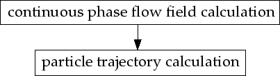
For the uncoupled calculation, you will perform the following two steps:

1.   Solve the continuous phase flow field.

2.   Plot (and report) the particle trajectories for discrete phase injections of interest.

In the uncoupled approach, this two-step procedure completes the modeling effort, as illustrated in Figure  23.6.1. The particle trajectories are computed as they are displayed, based on a fixed continuous-phase flow field. Graphical and reporting options are detailed in Section  23.7.

Figure 23.6.1: Uncoupled Discrete Phase Calculations

This procedure is adequate when the discrete phase is present at a low mass and momentum loading, in which case the continuous phase is not impacted by the presence of the discrete phase.

Coupled Calculations

In a coupled two-phase simulation, ANSYS FLUENT modifies the two-step procedure above as follows:

1.   Solve the continuous phase flow field (prior to introduction of the discrete phase).

2.   Introduce the discrete phase by calculating the particle trajectories for each discrete phase injection.

3.   Recalculate the continuous phase flow, using the interphase exchange of momentum, heat, and mass determined during the previous particle calculation.

4.   Recalculate the discrete phase trajectories in the modified continuous phase flow field.

5.   Repeat the previous two steps until a converged solution is achieved in which both the continuous phase flow field and the discrete phase particle trajectories are unchanged with each additional calculation.

This coupled calculation procedure is illustrated in Figure  23.6.2. When your ANSYS FLUENT model includes a high mass and/or momentum loading in the discrete phase, the coupled procedure must be followed in order to include the important impact of the discrete phase on the continuous phase flow field.

Figure 23.6.2: Coupled Discrete Phase Calculations

When you perform coupled calculations, all defined discrete phase injections will be computed. You cannot calculate a subset of the injections you have defined. If there are massless particle injections defined, these will have no effect in the coupled calculation.

Procedures for a Coupled Two-Phase Flow

If your ANSYS FLUENT model includes prediction of a coupled two-phase flow, you should begin with a partially (or fully) converged continuous-phase flow field. You will then create your injection(s) and set up the coupled calculation.

For each discrete-phase iteration, ANSYS FLUENT computes the particle/droplet trajectories and updates the interphase exchange of momentum, heat, and mass in each control volume. These interphase exchange terms then impact the continuous phase when the continuous phase iteration is performed. During the coupled calculation, ANSYS FLUENT will perform the discrete phase iteration at specified intervals during the continuous-phase calculation. The coupled calculation continues until the continuous phase flow field no longer changes with further calculations (i.e., all convergence criteria are satisfied). When convergence is reached, the discrete phase trajectories no longer change either, since changes in the discrete phase trajectories would result in changes in the continuous phase flow field.

The steps for setting up the coupled calculation are as follows:

1.   Solve the continuous phase flow field.

2.   In the Discrete Phase Model dialog box (Figure  23.2.1), enable the Interaction with Continuous Phase option.

3.   Set the frequency with which the particle trajectory calculations are introduced in the Number of Continuous Phase Iterations Per DPM Iteration field. If you set this parameter to 5, for example, a discrete phase iteration will be performed every fifth continuous phase iteration. The optimum number of iterations between trajectory calculations depends upon the physics of your ANSYS FLUENT model.

Note that if you set this parameter to 0, ANSYS FLUENT will not perform any discrete phase iterations.

During the coupled calculation (which you initiate using the Run Calculation task page in the usual manner) you will see the following information in the ANSYS FLUENT console as the continuous and discrete phase iterations are performed:

iter continuity x-velocity y-velocity          k    epsilon     energy time/it
 314 2.5249e-01 2.8657e-01 1.0533e+00 7.6227e-02 2.9771e-02 9.8181e-03 :00:05
 315 2.7955e-01 2.5867e-01 9.2736e-01 6.4516e-02 2.6545e-02 4.2314e-03 :00:03

DPM Iteration ....
number tracked= 9, number escaped= 1, aborted= 0, trapped= 0, evaporated = 8,i
Done.
 316 1.9206e-01 1.1860e-01 6.9573e-01 5.2692e-02 2.3997e-02 2.4532e-03 :00:02
 317 2.0729e-01 3.2982e-02 8.3036e-01 4.1649e-02 2.2111e-02 2.5369e-01 :00:01
 318 3.2820e-01 5.5508e-02 6.0900e-01 5.9018e-02 2.6619e-02 4.0394e-02 :00:00

Note that you can perform a discrete phase calculation at any time by using the solve/dpm-update text command.

Stochastic Tracking in Coupled Calculations

If you include the stochastic prediction of turbulent dispersion in the coupled two-phase flow calculations, the number of stochastic tries applied each time the discrete phase trajectories are introduced during coupled calculations will be equal to the Number of Tries specified in the Set Injection Properties dialog box. Input of this parameter is described in Section  23.3.16.

Note that the number of tries should be set to 0 if you want to perform the coupled calculation based on the mean continuous phase flow field. An input of $n \geq 1$ requests $n$ stochastic trajectory calculations for each particle in the injection. Note that when the number of stochastic tracks included is small, you may find that the ensemble average of the trajectories is quite different each time the trajectories are computed. These differences may, in turn, impact the convergence of your coupled solution. For this reason, you should include an adequate number of stochastic tracks in order to avoid convergence troubles in coupled calculations.

Under-Relaxation of the Interphase Exchange Terms

When you are coupling the discrete and continuous phases for steady-state calculations, using the calculation procedures noted above, ANSYS FLUENT applies under-relaxation to the momentum, heat, and mass transfer terms. This under-relaxation serves to increase the stability of the coupled calculation procedure by letting the impact of the discrete phase change only gradually:

where $E_{\rm new}$ is the exchange term, $E_{\rm old}$ is the previous value, $E_{\rm calculated}$ is the newly computed value, and $\alpha$ is the particle/droplet under-relaxation factor. ANSYS FLUENT uses a default value of 0.5 for $\alpha$. You can modify $\alpha$ by changing the value in the Discrete Phase Sources field under Under-Relaxation Factors in the Solution Controls task page. You may need to decrease $\alpha$ in order to improve the stability of coupled discrete phase calculations.

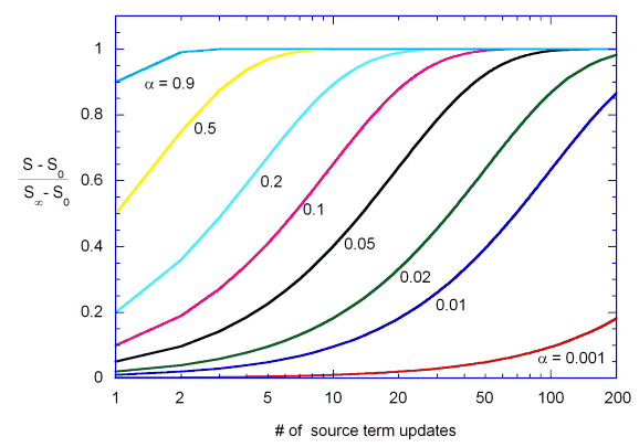
Figure  23.6.3 shows how the source term, $S$, when applied to the flow equations, changes with the number of updates for varying under-relaxation factors. In Figure  23.6.3, $S_{\infty}$ is the final source term for which a value is reached after a certain number of updates and $S_0$ is the initial source term at the start of the computation. The value of $S_0$ is typically zero at the beginning of the calculation.

Figure 23.6.3: Effect of Number of Source Term Updates on Source Term Applied to Flow Equations

Figure  23.6.3 can be applied to this option as well. Keep in mind that the DPM source terms are updated every continuous flow iteration.