7.6.4 Reorienting Profiles

For 3D cases only, ANSYS FLUENT allows you to change the orientation of an existing profile so that it can be used at a boundary positioned arbitrarily in space. This allows you, for example, to take experimental data for an inlet with one orientation and apply it to an inlet in your model that has a different spatial orientation. Note that ANSYS FLUENT assumes that the profile and the boundary are planar.

Steps for Changing the Profile Orientation

The procedure for orienting the profile data in the principal directions of a boundary is outlined below:

1.   Define and read the profile as described in Section  7.6.3.

2.   In the Profiles dialog box, select the profile in the Profile list, and then click the Orient... button. This will open the Orient Profile dialog box (Figure  7.6.3).

Figure 7.6.3: The Orient Profile Dialog Box

3.   In the Orient Profile dialog box, enter the name of the new profile you want to create in the New Profile box.

4.   Specify the number of fields you want to create using the up/down arrows next to the New Fields box. The number of new fields is equal to the number of vectors and scalars to be defined plus 1 (for the coordinates).

5.   Define the coordinate field.

(a)   Enter the names of the three coordinates ( $x$, $y$, $z$) in the first row under New Field Names.

Ensure that the coordinates are named $x$, $y$, and $z$ only. Do not use any other names or upper case letters in this field.

(b)   Select the appropriate local coordinate fields for $x$, $y$, and $z$ from the drop-down lists under Compute From.... (A selection of 0 indicates that the coordinate does not exist in the original profile; i.e., the original profile was defined in 2D.)

6.   Define the vector fields in the new profile.

(a)   Enter the names of the 3 components in the directions of the coordinate axes of the boundary under New Field Names.

Do not use upper case letters in these fields.

(b)   Select the names of the 3 components of the vector in the local $x$, $y$, and $z$ directions of the profile from the drop-down lists under Compute From....

7.   Define the scalar fields in the new profile.

(a)   Enter the name of the scalar in the first column under New Field Names.

Do not use upper case letters in these fields.

(b)   Click the button under Treat as Scalar Quantity in the same row.

(c)   Select the name of the scalar in the corresponding drop-down list under Compute From....

8.   Under Orient To..., specify the rotational matrix $RM$ under the Rotation Matrix [RM]. The rotational matrix used here is based on Euler angles ( $\gamma$, $\beta$, and $\alpha$) that define an orthogonal system $x'y'z'$ as the result of the three successive rotations from the original system $xyz$. In other words,

where C, B, and A are the successive rotations around the $z$, $y$, and $x$ axes, respectively.

Rotation around the $z$ axis:

Rotation around the $y$ axis:

Rotation around the $x$ axis:

9.   Under Orient To..., specify the Direction Vector. The Direction Vector is the vector that translates a profile to the new position, and is defined between the centers of the profile fields.

Note that depending on your case, it may be necessary to perform only a rotation, only a translation, or a combination of a translation and a rotation.

10.   Click the Create button in the Orient Profile dialog box, and your new profile will be created. Its name, which you entered in the New Profile box, will now appear in the Profiles dialog box and will be available for use at the desired boundary.

Profile Orienting Example

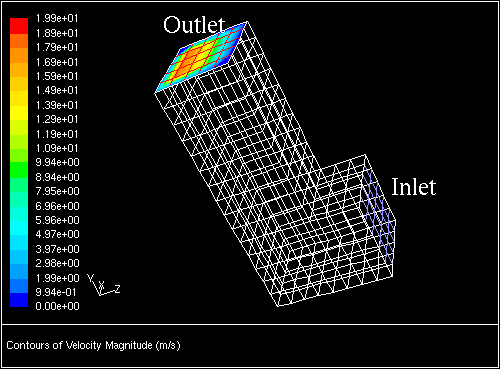
Consider the domain with a square inlet and outlet, shown in Figure  7.6.4. A scalar profile at the outlet is written out to a profile file. The purpose of this example is to impose this outlet profile on the inlet boundary via a 90 $^\circ$ rotation about the $x$ axis. However, the rotation will locate the profile away from the inlet boundary. To align the profile to the inlet boundary, a translation via a directional vector needs to be performed.

Figure 7.6.4: Scalar Profile at the Outlet

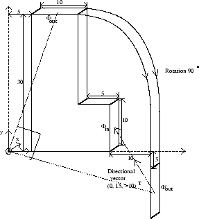
The problem is shown schematically in Figure  7.6.5. $\Phi_{\rm out}$ is the scalar profile of the outlet. $\Phi'_{\rm out}$ is the image of the $\Phi_{\rm out}$ rotated 90 $^\circ$ around the $x$ axis. In this example, since $\gamma = \beta = 0$, then $C = B = I$, where $I$ is the identity matrix, and the rotation matrix is

To overlay the outlet profile on the inlet boundary, a translation will be performed. The directional vector is the vector that translates $\Phi'_{\rm out}$ to $\Phi_{\rm in}$. In this example, the directional vector is 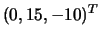$(0, 15, -10)^T$. The appropriate inputs for the Orient Profile dialog box are shown in Figure  7.6.3.

Note that if the profile being imposed on the inlet boundary was due to a rotation of -90 $^\circ$ about the $x$ axis, then the rotational matrix $RM$ must be found for $\gamma = \beta = 0$ and $\alpha = -90^\circ$, and a new directional vector must be found to align the profile to the boundary.

Figure 7.6.5: Problem Specification