7.4.1 Turbo-Specific Non-Reflecting Boundary Conditions

Overview

The standard pressure boundary conditions for compressible flow fix specific flow variables at the boundary (e.g., static pressure at an outlet boundary). As a result, pressure waves incident on the boundary will reflect in an unphysical manner, leading to local errors. The effects are more pronounced for internal flow problems where boundaries are usually close to geometry inside the domain, such as compressor or turbine blade rows.

The turbo-specific non-reflecting boundary conditions permit waves to "pass'' through the boundaries without spurious reflections. The method used in ANSYS FLUENT is based on the Fourier transformation of solution variables at the non-reflecting boundary [ 26]. Similar implementations have been investigated by other authors [ 52, 68]. The solution is rearranged as a sum of terms corresponding to different frequencies, and their contributions are calculated independently. While the method was originally designed for axial turbomachinery, it has been extended for use with radial turbomachinery.

Limitations

Note the following limitations of turbo-specific NRBCs:

• They are available only with the density-based solver (explicit or implicit).

• The current implementation applies to steady compressible flows, with the density calculated using the ideal gas law.

• Inlet and outlet boundary conditions must be pressure inlets and outlets only.

  Note that the pressure inlet boundaries must be set to the cylindrical coordinate flow specification method when turbo-specific NRBCs are used.

• Quad-mapped (structured) surface meshes must be used for inflow and outflow boundaries in a 3D geometry (i.e., triangular or quad-paved surface meshes are not allowed). See Figures  7.4.1 and 7.4.2 for examples.

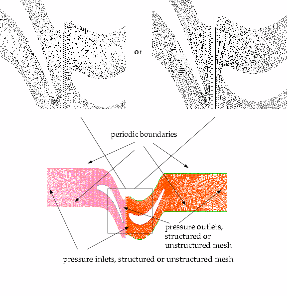
  Note that you may use unstructured meshes in 2D geometries (Figure  7.4.3), and an unstructured mesh may be used away from the inlet and outlet boundaries in 3D geometries.

• The turbo-specific NRBC method used in ANSYS FLUENT is based on quasi-3D analysis. The method developed for 2D turbo-specific NRBC [ 26] has been extended for use on 3D geometries [ 68] by decoupling the tangential flow variations from the radial variations. This approximation works best for geometries with a blade pitch that is small compared to the radius of the geometry.

• Reverse flow on the inflow and outflow boundaries are not allowed. If strong reverse flow is present, then you should consider using the General NRBCs instead.

• NRBCs are not compatible with species transport models. They are mainly used to solve ideal-gas single-species flow.

Figure 7.4.1: Mesh and Prescribed Boundary Conditions in a 3D Axial Flow Problem

Figure 7.4.2: Mesh and Prescribed Boundary Conditions in a 3D Radial Flow Problem

Figure 7.4.3: Mesh and Prescribed Boundary Conditions in a 2D Case

Theory

Turbo-specific NRBCs are based on Fourier decomposition of solutions to the linearized Euler equations. The solution at the inlet and outlet boundaries is circumferentially decomposed into Fourier modes, with the 0th mode representing the average boundary value (which is to be imposed as a user input), and higher harmonics that are modified to eliminate reflections [ 68].

Equations in Characteristic Variable Form

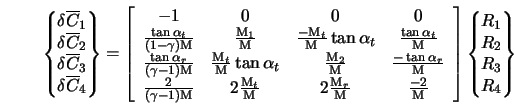
In order to treat individual waves, the linearized Euler equations are transformed to characteristic variable ( $C_i$) form. If we first consider the 1D form of the linearized Euler equations, it can be shown that the characteristic variables $C_i$ are related to the solution variables as follows:

where

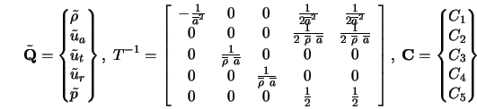
where $\overline{a}$ is the average acoustic speed along a boundary zone, $\tilde{\rho}$, $\tilde{u}_a$, $\tilde{u}_t$, $\tilde{u}_r$, and $\tilde{p}$ represent perturbations from a uniform condition (e.g., 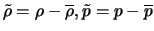$\tilde{\rho} = \rho - \overline{\rho}, \tilde{p} = p - \overline{p}$, etc.).

Note that the analysis is performed using the cylindrical coordinate system. All overlined (averaged) flow field variables (e.g., $\overline{\rho}$, $\overline{a}$) are intended to be averaged along the pitchwise direction.

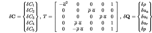
In quasi-3D approaches [ 26, 52, 68], a procedure is developed to determine the changes in the characteristic variables, denoted by $\delta C_i$, at the boundaries such that waves will not reflect. These changes in characteristic variables are determined as follows:

where

The changes to the outgoing characteristics -- one characteristic for subsonic inflow ( $\delta C_5$), and four characteristics for subsonic outflow ( $\delta C_1$, $\delta C_2$, $\delta C_3$, $\delta C_4$) -- are determined from extrapolation of the flow field variables using Equation  7.4-2.

The changes in the incoming characteristics -- four characteristics for subsonic inflow ( $\delta C_1$, $\delta C_2$, $\delta C_3$, $\delta C_4$), and one characteristic for subsonic outflow ( $\delta C_5$) -- are split into two components: average change along the boundary ( $\delta \overline{C}_i$), and local changes in the characteristic variable due to harmonic variation along the boundary ( $\delta C_{iL}$). The incoming characteristics are therefore given by

where $i = 1,2,3,4$ on the inlet boundary or $i = 5$ on the outlet boundary, and $j = 1, ..., N$ is the grid index in the pitchwise direction including the periodic point once. The under-relaxation factor $\sigma$ has a default value of $0.75$. Note that this method assumes a periodic solution in the pitchwise direction.

The flow is decomposed into mean and circumferential components using Fourier decomposition. The 0th Fourier mode corresponds to the average circumferential solution, and is treated according to the standard 1D characteristic theory. The remaining parts of the solution are described by a sum of harmonics, and treated as 2D non-reflecting boundary conditions [ 26].

Inlet Boundary

For subsonic inflow, there is one outgoing characteristic ( $\delta C_5$) determined from Equation  7.4-2, and four incoming characteristics ( $\delta C_1$, $\delta C_2$, $\delta C_3$, $\delta C_4$) calculated using Equation  7.4-3. The average changes in the incoming characteristics are computed from the requirement that the entropy ( $s$), radial and tangential flow angles ( $\alpha_r$ and $\alpha_t$), and stagnation enthalpy ( $h_0$) are specified. 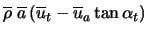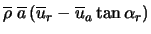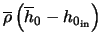Note that in ANSYS FLUENT you can specify $p_0$ and $T_0$ at the inlet, from which $s_{{\rm in}}$ and $h_{0_{\rm in}}$ are easily obtained. This is equivalent to forcing the following four residuals to be zero:

$$R_1 = \overline{p} \left(\overline{s} - s_{{\rm in}} \right)$$ (7.4-5)

$$R_2 = \overline{\rho}\mbox{ }\overline{a} \left(\overline{u}_t - \overline{u}_a \tan{\alpha_t} \right)$$ (7.4-6)

$$R_3 = \overline{\rho}\mbox{ }\overline{a} \left(\overline{u}_r - \overline{u}_a \tan{\alpha_r} \right)$$ (7.4-7)

$$R_4 = \overline{\rho} \left(\overline{h}_0 - h_{0_{\rm in}} \right)$$ (7.4-8)

where

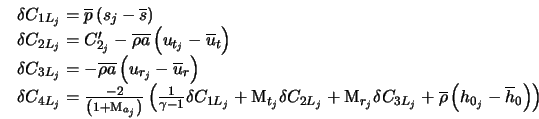
The average characteristic is then obtained from residual linearization as follows (see also Figure  7.4.4 for an illustration of the definitions for the prescribed inlet angles):

where

$${\rm M_a} = \frac{\overline{u}_a}{\overline{a}}$$ (7.4-12)

$${\rm M_t} = \frac{\overline{u}_t}{\overline{a}}$$ (7.4-13)

$${\rm M_r} = \frac{\overline{u}_r}{\overline{a}}$$ (7.4-14)

and

Figure 7.4.4: Prescribed Inlet Angles

where

$$e_t = \frac{u_t}{\vert v\vert}$$ (7.4-19)

$$e_r = \frac{u_r}{\vert v\vert}$$ (7.4-20)

$$e_a = \frac{u_a}{\vert v\vert}$$ (7.4-21)

To address the local characteristic changes at each $j$ grid point along the inflow boundary, the following relations are developed [ 26, 68]:

Note that the relation for the first and fourth local characteristics force the local entropy and stagnation enthalpy to match their average steady-state values.

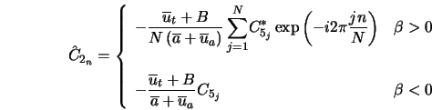
The characteristic variable $C'_{2_j}$ is computed from the inverse discrete Fourier transform of the second characteristic. The discrete Fourier transform of the second characteristic in turn is related to the discrete Fourier transform of the fifth characteristic. Hence, the characteristic variable $C'_{2_j}$ is computed along the pitch as follows:

The Fourier coefficients $C'_{2_n}$ are related to a set of equidistant distributed characteristic variables $C_{5_j}^{*}$ by the following [ 52]:

where

and

The set of equidistributed characteristic variables $C_{5_j}^{*}$ is computed from arbitrary distributed $C_{5_j}$ by using a cubic spline for interpolation, where

For supersonic inflow the user-prescribed static pressure ( $p_{s_{\rm in}}$) along with total pressure ( $p_{0_{\rm in}}$) and total temperature ( $T_{0_{\rm in}}$) are sufficient for determining the flow condition at the inlet.

Outlet Boundary

For subsonic outflow, there are four outgoing characteristics ( $\delta C_1$, $\delta C_2$, $\delta C_3$, and $\delta C_4$) calculated using Equation  7.4-2, and one incoming characteristic ( $\delta C_5$) determined from Equation  7.4-3. The average change in the incoming fifth characteristic is given by

where $\overline{p}$ is the current averaged pressure at the exit plane and $p_{\rm out}$ is the desirable average exit pressure (this value is specified by you for single-blade calculations or obtained from the assigned profile for mixing-plane calculations). The local changes ( $\delta C_{5L_j}$) are given by

The characteristic variable $C^{'}_{5_j}$ is computed along the pitch as follows:

The Fourier coefficients $\hat{C}_{5_n}$ are related to two sets of equidistantly distributed characteristic variables ( $C_{2_j}^{*}$ and $C_{4_j}^{*}$, respectively) and given by the following [ 52]:

where

The two sets of equidistributed characteristic variables ( $C_{2_j}^{*}$ and $C_{4_j}^{*}$) are computed from arbitrarily distributed $C_{2_j}$ and $C_{4_j}$ characteristics by using a cubic spline for interpolation, where

For supersonic outflow all flow field variables are extrapolated from the interior.

Updated Flow Variables

Once the changes in the characteristics are determined on the inflow or outflow boundaries, the changes in the flow variables $\delta {\bf Q}$ can be obtained from Equation  7.4-2. Therefore, the values of the flow variables at the boundary faces are as follows:

$$p_f = p_j + \delta p$$ (7.4-38)

$$u_{a_f} = u_{a_j} + \delta u_a$$ (7.4-39)

$$u_{t_f} = u_{t_j} + \delta u_t$$ (7.4-40)

$$u_{r_f} = u_{r_j} + \delta u_r$$ (7.4-41)

$$T_f = T_j + \delta T$$ (7.4-42)

Using Turbo-Specific Non-Reflecting Boundary Conditions

If you intend to use turbo-specific NRBCs in conjunction with the density-based implicit solver, it is recommended that you first converge the solution before turning on turbo-specific NRBCs, then converge it again with turbo-specific NRBCs turned on. If the solution is diverging, then you should lower the CFL number. These steps are necessary because only approximate flux Jacobians are used for the pressure-inlet and pressure-outlet boundaries when turbo-specific NRBCs are activated with the density-based implicit solver.

The procedure for using the turbo-specific NRBCs is as follows:

1.   Turn on the turbo-specific NRBCs using the non-reflecting-bc text command:

define $\rightarrow$ boundary-conditions $\rightarrow$ non-reflecting-bc $\rightarrow$ turbo-specific-nrbc $\rightarrow$ enable?

If you are not sure whether or not NRBCs are turned on, use the show-status text command.

2.   Perform NRBC initialization using the initialize text command:

define $\rightarrow$ boundary-conditions $\rightarrow$ non-reflecting-bc $\rightarrow$ turbo-specific-nrbc $\rightarrow$ initialize

If the initialization is successful, a summary printout of the domain extent will be displayed. If the initialization is not successful, an error message will be displayed indicating the source of the problem. The initialization will set up the pressure-inlet and pressure-outlet boundaries for use with turbo-specific NRBCs.

Note that the pressure inlet boundaries must be set to the cylindrical coordinate flow specification method when turbo-specific NRBCs are used.

3.   If necessary, modify the parameters in the set/ submenu:

define $\rightarrow$ boundary-conditions $\rightarrow$ non-reflecting-bc $\rightarrow$ turbo-specific-nrbc $\rightarrow$ set

under-relaxation   allows you to set the value of the under-relaxation factor $\sigma$ in Equation  7.4-3. The default value is $0.75$.

discretization   allows you to set the discretization scheme. The default is to use higher-order reconstruction if available.

verbosity   allows you to control the amount of information printed to the console during an NRBC calculation.

• 0 : silent

• 1 : basic information (default)

• 2 : detailed information (for debugging purposes only)

Using the NRBCs with the Mixing-Plane Model

If you want to use the NRBCs with the mixing-plane model you must define the mixing plane interfaces as pressure-outlet and pressure-inlet zone type pairs.

Turbo-specific NRBCs should not be used with the mixing-plane model if reverse flow is present across the mixing-plane.

Using the NRBCs in Parallel ANSYS FLUENT

When the turbo-specific NRBCs are used in conjunction with the parallel solver, all cells in each boundary zone, where NRBCs will be applied, must be located or contained within a single partition. You can ensure this by manually partitioning the mesh (see Section  32.5.4 for more information).