![[ANSYS, Inc. Logo]](fluentlogo.gif)


|
|
|
Some flows may contain flow features that are easy to identify based on values of a certain quantity. For instance, wakes represent a total pressure deficit, and jets are identifiable by a region of relatively high-velocity fluid. Since it is known that these regions also contain large gradients of important flow quantities (such as
 and
and
 in turbulent flows), it is convenient to perform an isovalue adaption on the relevant flow quantity than to refine on gradients of the individual flow variables.
The isovalue adaption function allows you to mark or refine cells inside or outside a specified range of a selected field variable function. The mesh can be refined or marked for refinement based on geometric and/or solution vector data. Specifically, any quantity in the display list of field variables can be used for the isovalue adaption. Some examples of how you might use the isovalue marking/adaption feature include the following:
 coordinate, etc.), and then visit each cell, marking for refinement the cells that have values inside (or outside) the specified ranges.
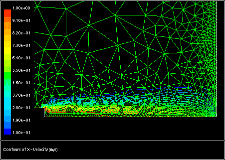
An example of a problem in which isovalue adaption is useful is shown in Figure
19.5.1. The mesh for an impinging jet is displayed along with contours of
 velocity. An isovalue adaption based on
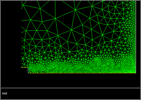
 velocity allows refinement of the mesh only in the jet (Figure
19.5.2).
velocity allows refinement of the mesh only in the jet (Figure
19.5.2).
Previous:
19.4 Dynamic Gradient Adaption