Step 10: Saving and Postprocessing Time-Dependent Data Sets

  At this point, the solution has reached a time-periodic state. To study how the flow changes within a single pressure cycle, you will now continue the solution for 100 more time steps. You will use ANSYS FLUENT's solution animation feature to save contour plots of pressure and Mach number at each time step, and the autosave feature to save case and data files every 10 time steps. After the calculation is complete, you will use the solution animation playback feature to view the animated pressure and Mach number plots over time.

1.   Request the saving of case and data files every 10 time steps.

Calculation Activities (Autosave Every) Edit...

(a)   Enter 10 for Save Data File Every.

(b)   Select Each Time for When the Data File is Saved, Save the Case File.

(c)   Retain the default selection of time-step from the Append File Name with drop-down list.

(d)   Enter noz_anim for File Name.

  When ANSYS FLUENT saves a file, it will append the time step value to the file name prefix ( noz_anim). The standard extensions ( .cas and .dat) will also be appended. This will yield file names of the form noz_anim0640.cas and noz_anim0640.dat, where 0640 is the time step number.

Optionally, you can add the extension .gz to the end of the file name (e.g., noz_anim.gz), which will instruct ANSYS FLUENT to save the case and data files in compressed format, yielding file names of the form noz_anim0640.cas.gz.

(e)   Click OK to close the Autosave dialog box.

Extra:   If you have constraints on disk space, you can restrict the number of files saved by ANSYS FLUENT by enabling the Retain Only the Most Recent Files option and setting the Maximum Number of Data Files to a nonzero number.

2.   Create animation sequences for the nozzle pressure and Mach number contour plots.

Calculation Activities (Solution Animations) Create/Edit...

(a)   Set Animation Sequences to 2.

(b)   Enter pressure for the Name of the first sequence and mach-number for the second sequence.

(c)   Select Time Step from the When drop-down lists for both sequences.

  With the default value of $1$ for Every, this instructs ANSYS FLUENT to update the animation sequence at every time step.

(d)   Click the Define... button for pressure to open the associated Animation Sequence dialog box.

i.   Select In Memory from the Storage Type group box.

  The In Memory option is acceptable for a small 2D case such as this. For larger 2D or 3D cases, saving animation files with either the Metafile or PPM Image option is preferable, to avoid using too much of your machine's memory.

ii.   Set Window to 3 and click the Set button.

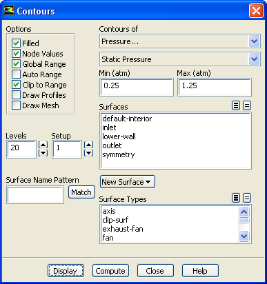
iii.   Select Contours from the Display Type group box to open the Contours dialog box.

a.   Make sure that Filled is enabled in the Options group box.

b.   Disable Auto Range.

c.   Retain the default selection of Pressure... and Static Pressure from the Contours of drop-down lists.

d.   Enter 0.25 atm for Min and 1.25 atm for Max.

  This will set a fixed range for the contour plot and subsequent animation.

e.   Click Display and close the Contours dialog box.

  Figure  4.7 shows the contours of static pressure in the nozzle after 600 time steps.

Figure 4.7: Pressure Contours at $t=0.017136$ s

iv.   Click OK to close the Animation Sequence dialog box associated with the pressure sequence.

(e)   Click the Define... button for mach-number to open the associated Animation Sequence dialog box.

i.   Make sure that In Memory is selected in the Storage Type list.

ii.   Set Window to 4 and click the Set button.

iii.   Select Contours in the Display Type group box to open the Contours dialog box.

a.   Select Velocity... and Mach Number from the Contours of drop-down lists.

b.   Make sure that Filled is enabled from the Options group box.

c.   Disable Auto Range.

d.   Enter 0.00 for Min and 1.30 for Max.

e.   Click Display and close the Contours dialog box.

  Figure  4.8 shows the Mach number contours in the nozzle after 600 time steps.

Figure 4.8: Mach Number Contours at $t=0.017136$ s

iv.   Click OK to close the Animation Sequence dialog box associated with the mach-number sequence.

(f)   Click OK to close the Solution Animation dialog box.

3.   Continue the calculation by requesting 100 time steps.

Run Calculation

  By requesting 100 time steps, you will march the solution through an additional 0.0028 seconds, or roughly one pressure cycle.

With the autosave and animation features active (as defined previously), the case and data files will be saved approximately every 0.00028 seconds of the solution time; animation files will be saved every 0.000028 seconds of the solution time.

  When the calculation finishes, you will have ten pairs of case and data files and there will be 100 pairs of contour plots stored in memory. In the next few steps, you will play back the animation sequences and examine the results at several time steps after reading in pairs of newly saved case and data files.

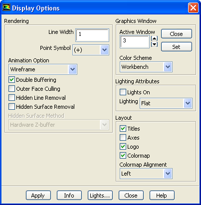
4.   Change the display options to include double buffering.

Graphics and Animations Options...

  Double buffering will allow for a smoother transition between the frames of the animations.

(a)   Enable the Double Buffering option.

(b)   Set Active Window to 3.

(c)   Click the Set button.

(d)   Click Apply and close the Display Options dialog box.

5.   Play the animation of the pressure contours.

Graphics and Animations Solution Animation Playback Set Up...

(a)   Retain the default selection of pressure in the Sequences selection list.

(b)   Click the play button (the second from the right in the group of buttons in the Playback group box).

(c)   Close the Playback dialog box.

  Examples of pressure contours at $t=0.017993$ s (the 630th time step) and $t=0.019135$ s (the 670th time step) are shown in Figures  4.9 and 4.10.

6.   In a similar manner to steps 4. and 5., select the appropriate active window and sequence name for the Mach number contours.

  Examples of Mach number contours at $t=0.017993$ s and $t=0.019135$ s are shown in Figures  4.11 and 4.12.

Figure 4.9: Pressure Contours at $t=0.017993$ s

Figure 4.10: Pressure Contours at $t=0.019135$ s

Figure 4.11: Mach Number Contours at $t=0.017993$ s

Figure 4.12: Mach Number Contours at $t=0.019135$ s

Extra:    ANSYS FLUENT gives you the option of exporting an animation as an MPEG file or as a series of files in any of the hardcopy formats available in the Save Picture dialog box (including TIFF and PostScript).

To save an MPEG file, select MPEG from the Write/Record Format drop-down list in the Playback dialog box and then click the Write button. The MPEG file will be saved in your working folder. You can view the MPEG movie using an MPEG player (e.g., Windows Media Player or another MPEG movie player).

To save a series of TIFF, PostScript, or other hardcopy files, select Picture Frames in the Write/Record Format drop-down list in the Playback dialog box. Click the Picture Options... button to open the Save Picture dialog box and set the appropriate parameters for saving the hardcopy files. Click Apply in the Save Picture dialog box to save your modified settings. In the Playback dialog box, click the Write button. ANSYS FLUENT will replay the animation, saving each frame to a separate file in your working folder.

If you want to view the solution animation in a later ANSYS FLUENT session, you can select Animation Frames as the Write/Record Format and click Write.

Since the solution animation was stored in memory, it will be lost if you exit ANSYS FLUENT without saving it in one of the formats described previously. Note that only the animation-frame format can be read back into the Playback dialog box for display in a later ANSYS FLUENT session.

7.   Read the case and data files for the 660th time step ( noz_anim0660.cas and noz_anim0660.dat) into ANSYS FLUENT.

8.   Plot vectors at $t=0.018849$ s (Figure  4.13).

Graphics and Animations Vectors Set Up...

(a)   Click Display and close the Vectors dialog box.

(b)   Select Auto Range under Options.

Figure 4.13: Velocity Vectors at $t=0.018849$ s

  The transient flow prediction in Figure  4.13 shows the expected form, with peak velocity of approximately 241 m/s through the nozzle at $t=0.018849$ seconds.

9.   In a similar manner to step 7. and 8., read the case and data files saved for other time steps of interest and display the vectors.