[ANSYS, Inc. Logo] return to home search
next up previous contents

Step 7: Solution

figure Solution

1.   Set the solution parameters.

figure Solution Methods

figure

(a)   Select Coupled from the Scheme drop-down list in the Pressure-Velocity Coupling group box.

(b)   Retain the default selection of Least Squares Cell Based from the Gradient drop-down list in the Spatial Discretization group box.

(c)   Retain the default selection of Standard from the Pressure drop-down list.

(d)   Select Second Order Upwind from the Density, Momentum, Modified Turbulent Viscosity, and Energy drop-down lists.

  Scroll down the Spatial Discretization group box to find the Energy drop-down list.

The second-order scheme will resolve the boundary layer and shock more accurately than the first-order scheme.

2.   Set the solution controls.

figure Solution Controls

figure

(a)   Retain the default value of 200 for Courant Number.

(b)   Enter 0.5 for Momentum and Pressure in the Explicit Relaxation Factors group box.

  Under-relaxing the momentum and pressure factors is recommended for higher-order discretization schemes.

(c)   Enter 0.5 for Density in the Under-Relaxation Factors group box.

  Under-relaxing the density factor is recommended for high-speed compressible flows.

(d)   Enter 0.9 for Modified Turbulent Viscosity.

  Larger under-relaxation factors (i.e., closer to 1) will generally result in faster convergence. However, instability can arise that may need to be eliminated by decreasing the under-relaxation factors.

3.   Enable residual plotting during the calculation.

figure Monitors figure figure Residuals figure Edit...

figure

(a)   Make sure that Plot is enabled in the Options group box and click OK to close the Residual Monitors dialog box.

4.   Initialize the solution.

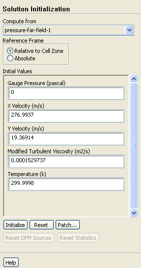
figure Solution Initialization

figure

(a)   Select pressure-far-field-1 from the Compute from drop-down list.

(b)   Click Initialize to initialize the solution.

(c)   Run the Full Multigrid (FMG) initialization.

  FMG initialization often facilitates an easier start-up, where no CFL ramping is necessary, thereby reducing the number of iterations for convergence.


i.   Press $<$ Enter $>$ in the console to get the command prompt ( $>$).

ii.   Enter the text commands and input responses as shown in the green. . Accept the default values by pressing $<$ Enter $>$ when no input response is given:

> solve/initialize/set-fmg-initialization


Customize your FMG initialization:
  set the number of multigrid levels [5] 

  set FMG parameters on levels .. 

   residual reduction on level 1 is:  [0.001] 
   number of cycles on level 1 is:  [10] 100


   residual reduction on level 2 is:  [0.001] 
   number of cycles on level 2 is:  [50] 100


   residual reduction on level 3 is:  [0.001] 
   number of cycles on level 3 is:  [100] 

   residual reduction on level 4 is:  [0.001] 
   number of cycles on level 4 is:  [500] 

   residual reduction on level 5 [coarsest grid] is:  [0.001] 
   number of cycles on level 5 is:  [500] 

 Number of FMG (and FAS  geometric multigrid) levels: 5 
* FMG customization summary: 
*   residual reduction on level 0 [finest grid] is: 0.001
*   number of cycles on level 0 is: 1
*   residual reduction on level 1 is: 0.001
*   number of cycles on level 1 is: 100
*   residual reduction on level 2 is: 0.001
*   number of cycles on level 2 is: 100
*   residual reduction on level 3 is: 0.001
*   number of cycles on level 3 is: 100
*   residual reduction on level 4 is: 0.001
*   number of cycles on level 4 is: 500
*   residual reduction on level 5 [coarsest grid] is: 0.001
*   number of cycles on level 5 is: 500
* FMG customization complete 

  set FMG courant-number [0.75] 

  enable FMG verbose? [no] yes


> solve/initialize/fmg-initialization

Enable FMG initialization? [no] yes

Note:   Whenever FMG initialization is performed, it is important to inspect the FMG initialized flow field using postprocessing tools of ANSYS FLUENT. Monitoring the normalized residuals, which are plotted in the console window will give you an idea of the convergence of the FMG solver. You should notice that the value of the normalized residuals decreases. For information about FMG initialization, including convergence strategies, see this section in the separate User's Guide.

5.   Save the case and data files ( airfoil.cas and airfoil.dat).

File $\rightarrow$ Write $\rightarrow$ Case & Data...

  It is good practice to save the case and data files during several stages of your case setup.

6.   Start the calculation by requesting 50 iterations.

figure Run Calculation

(a)   Enter 50 for Number of Iterations.

(b)   Click Calculate.

  By performing some iterations before setting up the force monitors, you will avoid large initial transients in the monitor plots. This will reduce the axes range and make it easier to judge the convergence.

7.   Set the reference values that are used to compute the lift, drag, and moment coefficients.

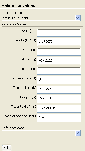
figure Reference Values

  The reference values are used to nondimensionalize the forces and moments acting on the airfoil. The dimensionless forces and moments are the lift, drag, and moment coefficients.

figure

(a)   Select pressure-far-field-1 from the Compute from drop-down list.

   ANSYS FLUENT will update the Reference Values based on the boundary conditions at the far-field boundary.

8.   Define a force monitor to plot and write the drag coefficient for the walls of the airfoil.

figure Monitors figure figure Drag figure Edit...

figure

(a)   Enable Plot in the Options group box.

(b)   Set Window to 3.

(c)   Enable Write to save the monitor history to a file.

Note:   If you do not enable the Write option, the history information will be lost when you exit ANSYS FLUENT.

(d)   Retain the default entry of cd-history for File Name.

(e)   Select wall-bottom and wall-top in the Wall Zones selection list.

(f)   Enter 0.9976 for X and 0.06976 for Y in the Force Vector group box.

  These X and Y values ensure that the drag coefficient is calculated parallel to the free-stream flow, which is $4^{\circ}$ off of the global coordinates.

(g)   Click OK to close the Drag Monitor dialog box.

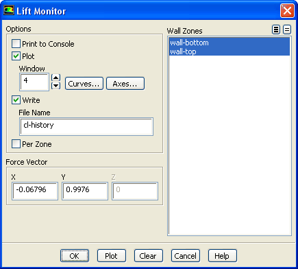
9.   Similarly, define a force monitor for the lift coefficient.

figure Monitors figure figure Lift figure Edit...

figure

  The X and Y values shown ensure that the lift coefficient is calculated normal to the free-stream flow, which is $4^{\circ}$ off of the global coordinates.

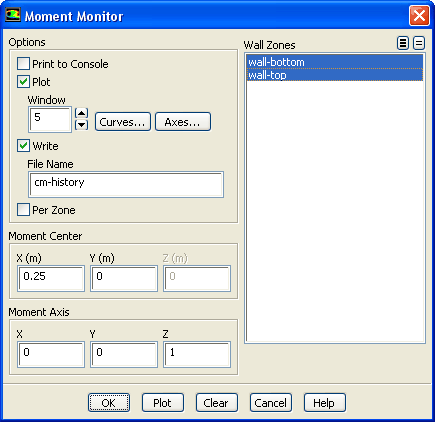
10.   In a similar manner, define a force monitor for the moment coefficient.

figure Monitors figure figure Moment figure Edit...

figure

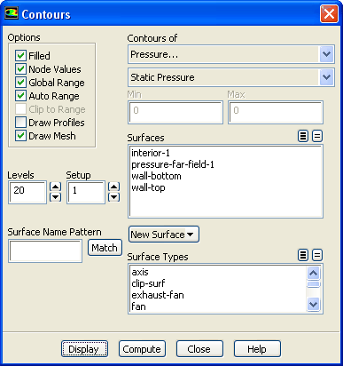
11.   Display filled contours of pressure overlaid with the mesh in preparation for defining a surface monitor (Figures  3.4 and 3.5).

figure Graphics and Animations figure figure Contours figure Set Up...

figure

(a)   Enable Filled in the Options group box.

(b)   Enable Draw Mesh to open the Mesh Display dialog box.

figure

i.   Retain the default settings.

ii.   Close the Mesh Display dialog box.

(c)   Click Display and close the Contours dialog box.

Figure 3.4: Pressure Contours After 50 Iterations
figure

  The shock is clearly visible on the upper surface of the airfoil, where the pressure jumps to a higher value downstream of the low pressure area.

Note:   The color indicating a high pressure area near the leading edge of the airfoil is obscured by the overlaid green mesh. To view this contour, simply disable the Draw Mesh option in the Contours dialog box and click Display.

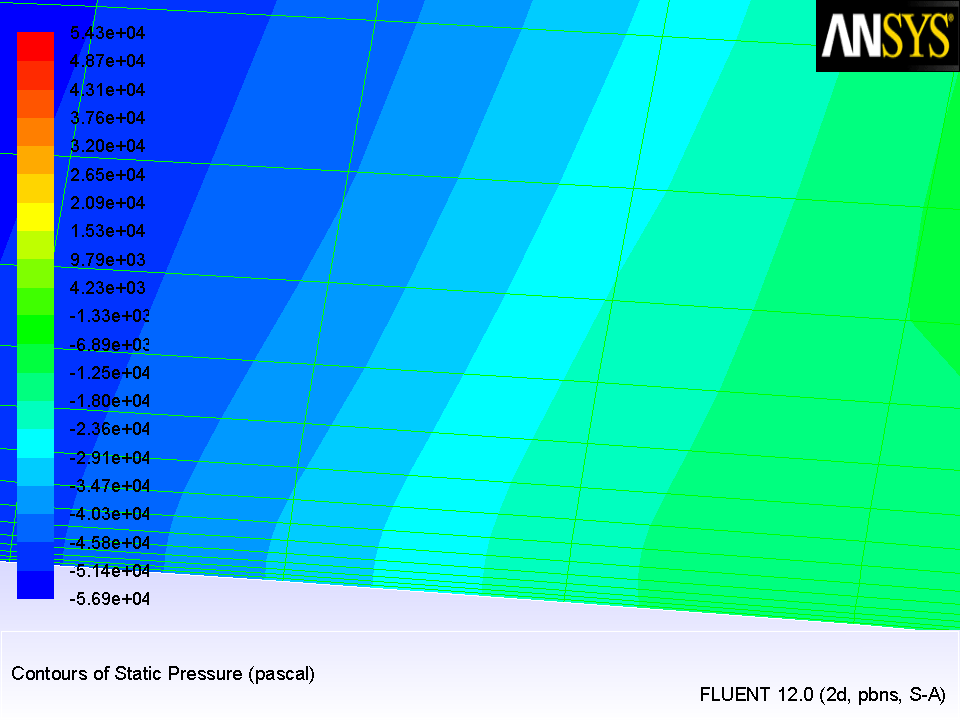
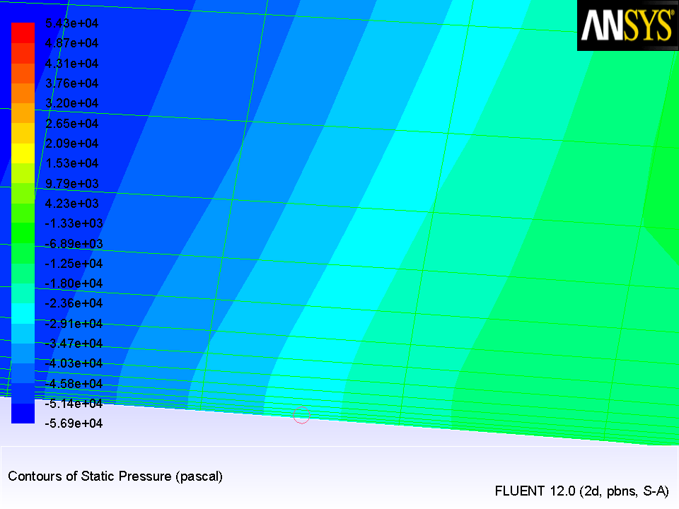
(d)   Zoom in on the shock wave, until individual cells adjacent to the upper surface ( wall-top boundary) are visible, as shown in Figure  3.5.

Figure 3.5: Magnified View of Pressure Contours Showing Wall-Adjacent Cells
figure

  The magnified region contains cells that are just downstream of the shock and adjacent to the upper surface of the airfoil. In the following step, you will create a point surface inside a wall-adjacent cell, which you will use to define a surface monitor.

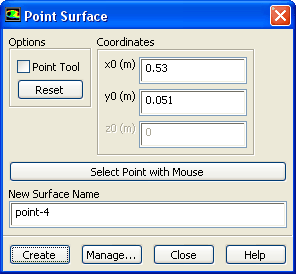
12.   Create a point surface just downstream of the shock wave.

Surface $\rightarrow$ Point...

figure

(a)   Enter 0.53 m for x0 and 0.051 m for y0 in the Coordinates group box.

(b)   Retain the default entry of point-4 for New Surface Name.

(c)   Click Create and close the Point Surface dialog box.

Note:   You have entered the exact coordinates of the point surface so that your convergence history will match the plots and description in this tutorial. In general, however, you will not know the exact coordinates in advance, so you will need to select the desired location in the graphics window as follows:

(a)   Click the Select Point with Mouse button.

(b)   Position the mouse pointer to a point located inside one of the cells adjacent to the upper surface ( wall-top boundary), downstream of the shock (see Figure  3.6).

(c)   Click the right mouse button.

(d)   Click Create to create the point surface and close the Point Surface dialog box.

Figure 3.6: Pressure Contours after Creating a Point with the Mouse
figure

13.   Enable residual plotting during the calculation.

figure Monitors figure figure Residuals figure Edit...

figure

(a)   Make sure that Plot is enabled in the Options group box.

(b)   Select none from the Convergence Criterion drop-down list so that automatic convergence checking does not occur.

(c)   Click OK to close the Residual Monitors dialog box.

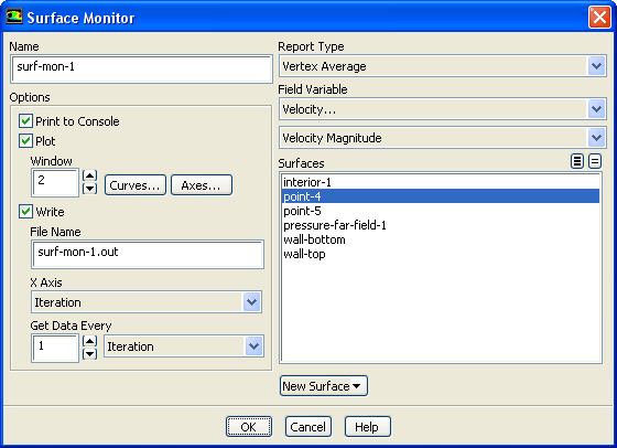
14.   Define a surface monitor for tracking the velocity magnitude value at the point created in the previous step.

  Since the drag, lift, and moment coefficients are global variables, indicating certain overall conditions, they may converge while local conditions at specific points are still varying from one iteration to the next. To account for this, define a monitor at a point (just downstream of the shock) where there is likely to be significant variation, and monitor the value of the velocity magnitude.

figure Monitors (Surface Monitors) figure Create...

figure

(a)   Enable Plot and Write.

(b)   Select Vertex Average from the Report Type drop-down list.

  Scroll down the Report Type drop-down list to find Vertex Average.

(c)   Select Velocity... and Velocity Magnitude from the Field Variable drop-down list.

(d)   Select point-4 in the Surfaces selection list.

(e)   Click OK to close the Surface Monitor dialog box.

15.   Save the case and data files ( airfoil-1.cas and airfoil-1.dat).

File $\rightarrow$ Write $\rightarrow$ Case & Data...

16.   Continue the calculation for 200 more iterations.

figure Run Calculation

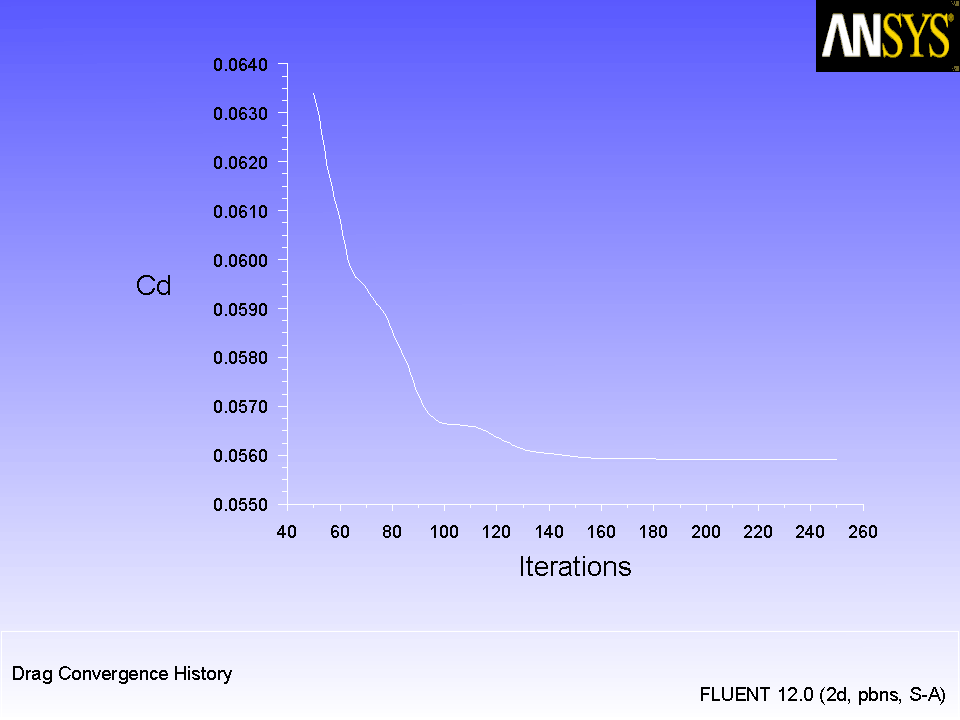
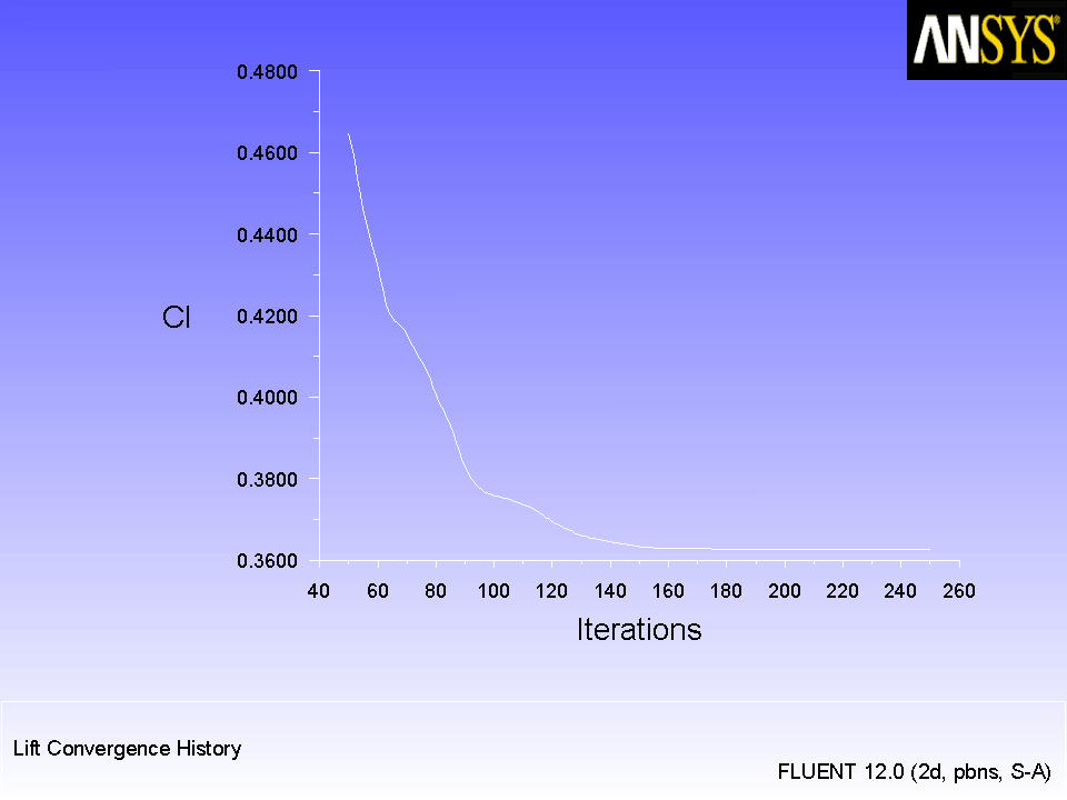
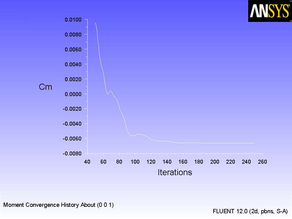
  The force monitors (Figures  3.8 and 3.9) show that the case is converged after approximately 200 iterations.

Figure 3.7: Velocity Magnitude History
figure

Figure 3.8: Drag Coefficient Convergence History
figure

Figure 3.9: Lift Coefficient Convergence History
figure

Figure 3.10: Moment Coefficient Convergence History
figure

17.   Save the case and data files ( airfoil-2.cas and airfoil-2.dat).

File $\rightarrow$ Write $\rightarrow$ Case & Data...


next up previous contents Previous: Step 6: Operating Conditions
Up: Modeling External Compressible Flow
Next: Step 8: Postprocessing
Release 12.0 © ANSYS, Inc. 2009-02-09