Step 9: Postprocessing

Graphics and Animations

1.   Display filled contours of static pressure (Figure  2.3).

Graphics and Animations Contours Set Up...

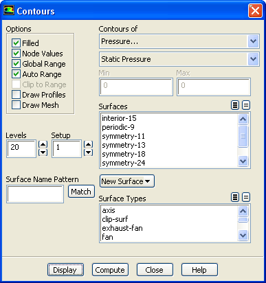
(a)   Enable Filled in the Options group box.

(b)   Retain the default selection of Pressure... and Static Pressure from the Contours of drop-down lists.

(c)   Click Display.

Figure 2.3: Contours of Static Pressure

(d)   Change the view to mirror the display across the symmetry planes (Figure  2.4).

Graphics and Animations Views...

i.   Select all of the symmetry zones ( symmetry-18, symmetry-13, symmetry-11, and symmetry-24) in the Mirror Planes selection list by clicking on the shaded icon in the upper right corner.

Note:   There are four symmetry zones in the Mirror Planes selection list because the top and bottom symmetry planes in the domain are each comprised of two symmetry zones, one on each side of the tube centered on the plane. It is also possible to generate the same display shown in Figure  2.4 by selecting just one of the symmetry zones on the top symmetry plane, and one on the bottom.

ii.   Click Apply and close the Views dialog box.

iii.   Translate the display of symmetry contours so that it is centered in the graphics window by using the left mouse button (Figure  2.4).

Figure 2.4: Contours of Static Pressure with Symmetry

  The pressure contours displayed in Figure  2.4 do not include the linear pressure gradient computed by the solver. Thus, the contours are periodic at the inlet and outflow boundaries.

2.   Display filled contours of static temperature (Figure  2.5).

Graphics and Animations Contours Set Up...

(a)   Select Temperature... and Static Temperature from the Contours of drop-down lists.

(b)   Click Display and close the Contours dialog box.

Figure 2.5: Contours of Static Temperature

  The contours in Figure  2.5 reveal the temperature increase in the fluid due to heat transfer from the tubes. The hotter fluid is confined to the near-wall and wake regions, while a narrow stream of cooler fluid is convected through the tube bank.

3.   Display the velocity vectors (Figure  2.6).

Graphics and Animations Vectors Set Up...

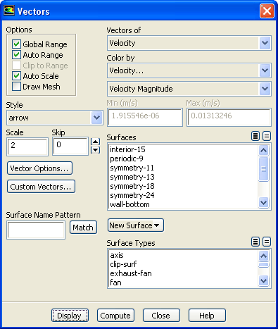
(a)   Enter 2 for Scale.

  This will increase the size of the displayed vectors, making it easier to view the flow patterns.

(b)   Retain the default selection of Velocity from the Vectors of drop-down list.

(c)   Retain the default selection of Velocity... and Velocity Magnitude from the Color by drop-down lists.

(d)   Click Display and close the Vectors dialog box.

(e)   Zoom in on the upper right portion of one of the left tubes to get the display shown in (Figure  2.6), by using the middle mouse button in the graphics window.

  The magnified view of the velocity vector plot in Figure  2.6 clearly shows the recirculating flow behind the tube and the boundary layer development along the tube surface.

Figure 2.6: Velocity Vectors

4.   Create an isosurface on the periodic tube bank at $x$ = 0.01 m (through the first column of tubes).

  This isosurface and the ones created in the steps that follow will be used for the plotting of temperature profiles.

Surface $\rightarrow$ Iso-Surface...

(a)   Select Mesh... and X-Coordinate from the Surface of Constant drop-down lists.

(b)   Enter 0.01 for Iso-Values.

(c)   Enter x=0.01m for New Surface Name.

(d)   Click Create.

5.   In a similar manner, create an isosurface on the periodic tube bank at $x$ = 0.02 m (halfway between the two columns of tubes) named x=0.02m.

6.   In a similar manner, create an isosurface on the periodic tube bank at $x$ = 0.03 m (through the middle of the second column of tubes) named x=0.03m, and close the Iso-Surface dialog box.

7.   Create an XY plot of static temperature on the three isosurfaces (Figure  2.7).

Plots XY Plot Set Up...

(a)   Enter 0 for X and 1 for Y in the Plot Direction group box.

  With a Plot Direction vector of (0,1), ANSYS FLUENT will plot the selected variable as a function of $y$. Since you are plotting the temperature profile on cross sections of constant $x$, the temperature varies with the $y$ direction.

(b)   Select Temperature... and Static Temperature from the Y-Axis Function drop-down lists.

(c)   Select x=0.01m, x=0.02m, and x=0.03m in the Surfaces selection list.

  Scroll down to find the x=0.01m, x=0.02m, and x=0.03m surfaces.

(d)   Click the Curves... button to open the Curves - Solution XY Plot dialog box.

  This dialog box is used to define plot styles for the different plot curves.

i.   Select $+$ from the Symbol drop-down list.

  Scroll up to find the $+$ item.

ii.   Click Apply to assign the $+$ symbol to the $x$ = 0.01 m curve.

iii.   Set the Curve # to 1 to define the style for the $x$ = 0.02 m curve.

iv.   Select x from the Symbol drop-down list.

  Scroll up to find the x item.

v.   Enter 0.5 for Size.

vi.   Click Apply and close the Curves - Solution XY Plot dialog box.

  Since you did not change the curve style for the $x$ = 0.03 m curve, the default symbol will be used.

(e)   Click Plot and close the Solution XY Plot dialog box.

Figure 2.7: Static Temperature at $x$=0.01, 0.02, and 0.03 m