Step 8: Solution

1.   Set the solution parameters.

Solution Methods

(a)   Retain the default setting of Least Squares Cell Based for the Gradient in the Spatial Discretization group box.

(b)   Select Second Order Upwind from the Momentum and Energy drop-down lists.

2.   Set the solution controls.

Solution Controls

(a)   Enter 0.9 for Energy in the Under-Relaxation Factors group box.

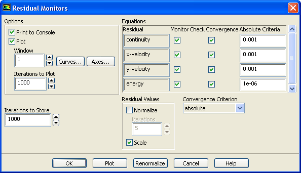
3.   Enable the plotting of residuals during the calculation.

Monitors Residuals Edit...

(a)   Make sure Plot is enabled in the Options group box.

(b)   Click OK to close the Residual Monitors dialog box.

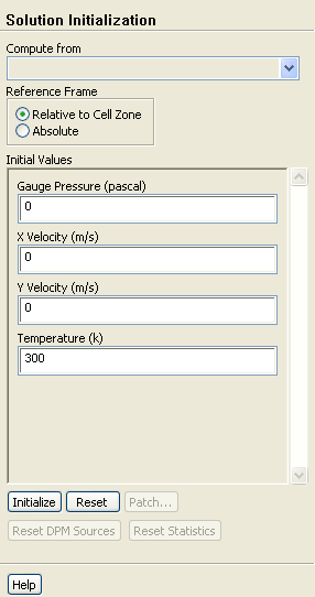
4.   Initialize the solution.

Solution Initialization

(a)   Retain the default setting of 300 K for Temperature in the Initial Values group box.

(b)   Click Initialize.

  The values shown in the task pane will be used as the initial condition for the solution.

5.   Save the case file ( tubebank.cas).

File $\rightarrow$ Write $\rightarrow$ Case...

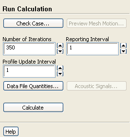
6.   Start the calculation by requesting 350 iterations.

Run Calculation

(a)   Enter 350 for Number of Iterations.

(b)   Click Calculate.

  The energy residual curve that is displayed in the graphics window will begin to flatten out as it approaches 350 iterations. For the solution to converge to the recommended residual value of $10^{-6}$, you need to reduce the under-relaxation factor for energy.

7.   Change the Under-Relaxation Factor for Energy to 0.6.

Solution Controls

8.   Continue the calculation by requesting another 300 iterations.

Run Calculation

  After restarting the calculation, the plot of the energy residual will display an initial dip as a result of the reduction of the under-relaxation factor. The solution will converge in a total of approximately 580 iterations.

9.   Save the case and data files ( tubebank.cas and tubebank.dat).

File $\rightarrow$ Write $\rightarrow$ Case & Data...