Step 10: Postprocessing

  In the next two steps you will examine the time-averaged values for the mass flow rates at the inlet and the outlet during the final revolution of the rotor. By comparing these values, you will verify the conservation of mass on a time-averaged basis for the system over the course of one revolution.

1.   Examine the time-averaged mass flow rate at the inlet during the final revolution of the rotor (as calculated from surf-mon-1c.out).

Plots FFT Set Up...

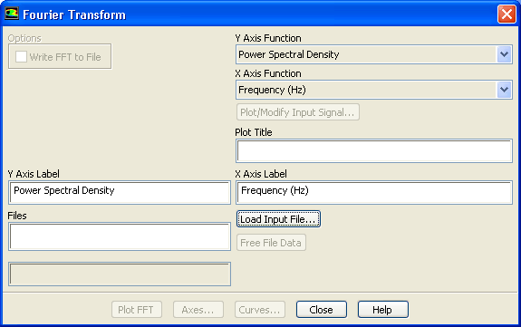
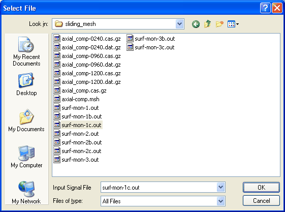
(a)   Click the Load Input File... button to open the Select File dialog box.

i.   Select All Files from the Files of type drop-down list.

ii.   Select surf-mon-1c.out from the list of files.

iii.   Click OK to close the Select File dialog box.

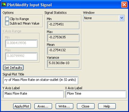
(b)   Click the Plot/Modify Input Signal... button to open the Plot/Modify Input Signal dialog box.

i.   Examine the values for Min, Max, Mean, and Variance in the Signal Statistics group box.

ii.   Close the Plot/Modify Input Signal dialog box.

(c)   Select the folder path ending in surf-mon-1c.out from the Files selection list.

(d)   Click the Free File Data button.

2.   Examine the time-averaged mass flow rate at the outlet during the final revolution of the rotor (as calculated from surf-mon-2c.out), and plot the data.

Plots FFT Set Up...

(a)   Click the Load Input File... button to open the Select File dialog box.

i.   Select All Files from the Files of type drop-down list.

ii.   Select surf-mon-2c.out from the list of files.

iii.   Click OK to close the Select File dialog box.

(b)   Click the Plot/Modify Input Signal... button to open the Plot/Modify Input Signal dialog box.

i.   Examine the values for Min, Max, Mean, and Variance in the Signal Statistics group box.

  The outlet mass flow rate values correspond very closely with those from the inlet, with the mean having approximately the same absolute value but with opposite signs. Thus, you can conclude that mass is conserved on a time-averaged basis during the final revolution of the rotor.

ii.   Click Set Defaults.

iii.   Click Apply/Plot to display the mass flow rate at the outlet (Figure  12.10).

Figure 12.10: Mass Flow Rate at the Outlet During the Final Revolution

iv.   Close the Plot/Modify Input Signal dialog box.

(c)   Close the Fourier Transform dialog box.

3.   Display contours of the mean static pressure on the walls of the axial compressor.

Graphics and Animations Contours Set Up...

(a)   Enable Filled in the Options group box.

(b)   Select Unsteady Statistics... and Mean Static Pressure from the Contours of drop-down lists.

(c)   Select wall from the Surface Types selection list.

  Scroll down the Surface Types selection list to find wall.

(d)   Click Display and close the Contours dialog box.

(e)   Rotate the view to get the display as shown in Figure  12.11.

  Shock waves are clearly visible in the flow near the outlets of the rotor and stator, as seen in the areas of rapid pressure change on the outer shroud of the axial compressor.

Figure 12.11: Mean Static Pressure on the Outer Shroud of the Axial Compressor