Step 9: Solution

1.   Set the solution parameters.

Solution Methods

(a)   Ensure that the Second Order Upwind is selected from the Flow drop-down list in the Spatial Discretization group box.

2.   Enable the plotting of residuals during the calculation.

Monitors Residuals Edit...

  

(a)   Ensure that the Plot is enabled in the Options group box.

(b)   Select relative from the Convergence Criterion drop-down list.

(c)   Enter 0.01 for Relative Criteria for each Residual ( continuity, x-velocity, y-velocity, z-velocity, and energy).

(d)   Click OK to close the Residual Monitors dialog box.

3.   Enable the plotting of mass flow rate at the inlet ( rotor-inlet).

Monitors (Surface Monitors) Create...

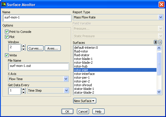
(a)   Retain the default entry of surf-mon-1 for Name.

(b)   Enable Plot and Write.

(c)   Retain the default entry of surf-mon-1.out for File Name.

(d)   Select Flow Time from the X Axis drop-down list.

(e)   Select Time Step from the Get Data Every drop-down list.

(f)   Select Mass Flow Rate from the Report Type drop-down list.

(g)   Select rotor-inlet from the Surfaces selection list.

(h)   Click OK to close the Surface Monitor dialog box.

4.   Enable the plotting of mass flow rate at the outlet ( stator-outlet).

Monitors (Surface Monitors) Create...

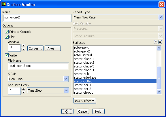
(a)   Retain the default entry of surf-mon-2 for Name.

(b)   Enable Plot and Write.

(c)   Retain the default entry of surf-mon-2.out for File Name.

(d)   Select Flow Time from the X Axis drop-down list.

(e)   Select Time Step from the Get Data Every drop-down list.

(f)   Select Mass Flow Rate from the Report Type drop-down list.

(g)   Select stator-outlet from the Surfaces selection list.

Ensure that the rotor-inlet is deselected from the Surfaces selection list before scrolling down to select stator-outlet.

(h)   Click OK to close the Surface Monitor dialog box.

5.   Enable the plotting of the area-weighted average of the static pressure at the interface ( stator-interface).

Monitors (Surface Monitors) Create...

(a)   Retain the default entry of surf-mon-3 for Name.

(b)   Enable Plot and Write.

(c)   Retain the default entry of surf-mon-3.out for File Name.

(d)   Select Flow Time from the X Axis drop-down list.

(e)   Select Time Step from the Get Data Every drop-down list.

(f)   Select Area-Weighted Average from the Report Type drop-down list.

(g)   Retain the default selection of Pressure... and Static Pressure from the Field Variable drop-down lists.

(h)   Select stator-interface from the Surfaces selection list.

Ensure that the stator-outlet is deselected from the Surfaces selection list before scrolling down to select stator-interface.

(i)   Click OK to close the Surface Monitor dialog box.

6.   Initialize the solution using the values at the inlet ( rotor-inlet).

Solution Initialization

(a)   Select rotor-inlet from the Compute from drop-down list.

(b)   Select Absolute in the Reference Frame list.

(c)   Click Initialize.

7.   Save the initial case file ( axial_comp.cas.gz).

File $\rightarrow$ Write $\rightarrow$ Case...

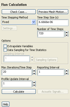
8.   Run the calculation for one revolution of the rotor.

Run Calculation

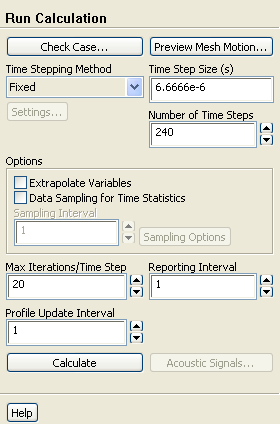
(a)   Enter 6.6666e-6 s for Time Step Size.

(b)   Enter 240 for Number of Time Steps.

  This time step represents the length of time during which the rotor will rotate 1.5 degrees. Since the periodic angle of the rotor is 22.5 degrees, the passing period of the rotor blade will equal 15 time steps, and a complete revolution of the rotor will take 240 time steps.

(c)   Retain the default setting of 20 for Max Iterations/Time Step.

(d)   Click Calculate.

  The calculation will run for approximately 3,700 iterations.

  The residuals jump at the beginning of each time step and then fall at least two to three orders of magnitude. Also, the relative convergence criteria is achieved before reaching the maximum iteration limit (20) for each time step, indicating the limit does not need to be increased.

Figure 12.3: Residual History for the First Revolution of the Rotor

9.   Examine the monitor histories for the first revolution of the rotor (Figures  12.4, 12.5, and 12.6).

Figure 12.4: Mass Flow Rate at the Inlet During the First Revolution

Figure 12.5: Mass Flow Rate at the Outlet During the First Revolution

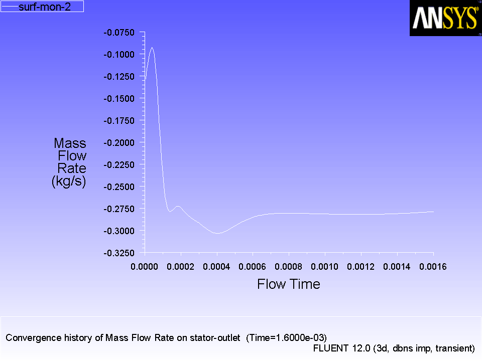Figure 12.6: Static Pressure at the Interface During the First Revolution

  The monitor histories show that the large variations in flow rate and interface pressure that occur early in the calculation are greatly reduced as time-periodicity is approached.

10.   Save the case and data files ( axial_comp-0240.cas.gz and axial_comp-0240.dat.gz).

File $\rightarrow$ Write $\rightarrow$ Case & Data...

It is a good practice to save the case file whenever you are saving the data file especially for sliding mesh model. This is because the case file contains the mesh information, which is changing with time.

Note:   For transient-state calculations, you can add the character string %t to the file name so that the iteration number is automatically appended to the name (e.g., by entering axial_comp-%t for the File Name in the Select File dialog box, ANSYS FLUENT will save files with the names axial_comp-0240.cas and axial_comp-0240.dat).

11.   Rename the monitor files in preparation for further iterations.

Monitors surf-mon-1 Edit...

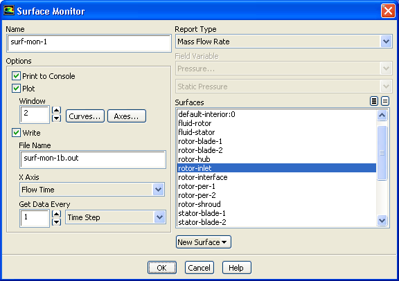
  By saving the monitor histories under a new file name, the range of the axes will automatically be set to show only the data generated during the next set of iterations. This will scale the plots so that the fluctuations are more visible.

(a)   Enter surf-mon-1b.out for File Name.

(b)   Click OK to close the Surface Monitor dialog box.

12.   Similarly, rename surf-mon-2.out and surf-mon-3.out to surf-mon-2b.out and
surf-mon-3b.out, respectively.

13.   Continue the calculation for 720 more time steps to simulate three more revolutions of the rotor.

Run Calculation

Calculating three more revolutions will require significant CPU resources. Instead of calculating the solution, you can read a data file ( axial_comp-0960.dat.gz) with the precalculated solution for this tutorial. This data file can be found in the sliding_mesh folder.

  The calculation will run for approximately 10,600 more iterations.

14.   Examine the monitor histories for the next three revolutions of the rotor to verify that the solution is time-periodic (Figures  12.7, 12.8, and 12.9).

Note:   If you read the provided data file instead of iterating the solution for three revolutions, the monitor histories can be displayed by using the File XY Plot dialog box.

Plots File Set Up...

Click the Add button in the File XY Plot dialog box to select one of the monitor histories from the Select File dialog box, click OK, and then click Plot.

Figure 12.7: Mass Flow Rate at the Inlet During the Next 3 Revolutions

Figure 12.8: Mass Flow Rate at the Outlet During the Next 3 Revolutions

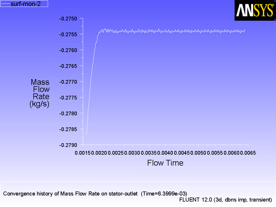Figure 12.9: Static Pressure at the Interface During the Next 3 Revolutions

Extra:   Note that the $Y$-axis for Figure  12.7 does not show enough significant figures to fully display the values of the mass flow rate.

15.   (Optional) Display the full values by using the File XY Plot dialog box.

Plots File Set Up...

(a)   Click the Add... button to open the Select File dialog box.

i.   Select surf-mon-1b.out and click OK to close the Select File dialog box.

(b)   Click the Axes... button to open the Axes - File XY Plot dialog box.

i.   Select Y in the Axis list.

ii.   Set Precision to 6.

iii.   Click Apply and close the Axes - File XY Plot dialog box.

(c)   Click Plot and close the File XY Plot dialog box.

16.   Save the case and data files ( axial_comp-0960.cas.gz and axial_comp-0960.dat.gz).

File $\rightarrow$ Write $\rightarrow$ Case & Data...

17.   Change the file names for surf-mon-1b.out, surf-mon-2b.out, and surf-mon-3b.out to surf-mon-1c.out, surf-mon-2c.out, and surf-mon-3c.out, respectively (as described in a previous step), in preparation for further iterations.

18.   Continue the calculation for one final revolution of the rotor, while saving data samples for the postprocessing of the time statistics.

Run Calculation

(a)   Enter 240 for Number of Time Steps.

(b)   Enable Data Sampling for Time Statistics in the Options group box.

(c)   Click Calculate.

  The calculation will run for approximately 3,400 more iterations.

19.   Save the case and data files ( axial_comp-1200.cas.gz and axial_comp-1200.dat.gz).

File $\rightarrow$ Write $\rightarrow$ Case & Data...