Step 7: Solution

1.   Set the solution parameters.

Solution Methods

(a)   Select Second Order Upwind from the Momentum, Turbulent Kinetic Energy, and Turbulent Dissipation Rate drop-down lists in the Spatial Discretization group box.

  The second-order scheme will provide a more accurate solution.

2.   Ensure the plotting of residuals during the calculation.

Monitors Residuals Edit...

(a)   Ensure that Plot is enabled in the Options group box.

(b)   Click OK to close the Residual Monitors dialog box.

3.   Initialize the solution using the boundary conditions set at pressure-inlet-5.

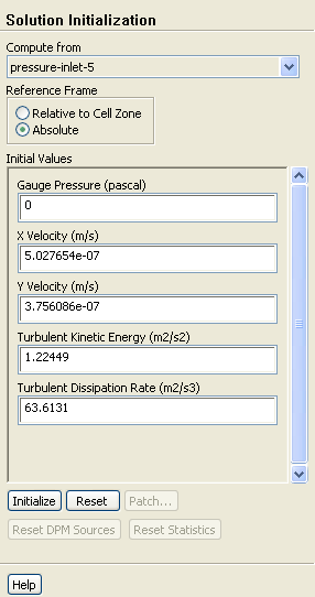
Solution Initialization

(a)   Select pressure-inlet-5 from the Compute from drop-down list.

(b)   Select Absolute in the Reference Frame list.

(c)   Click Initialize to initialize the solution.

Note:   In this tutorial, you chose an Absolute reference frame for initializing the solution. In certain cases, Relative to Cell Zone may help the solution converge faster.

For guidelines, see this section in the separate User's Guide.

4.   Save the case file ( blower.cas.gz).

File $\rightarrow$ Write $\rightarrow$ Case...

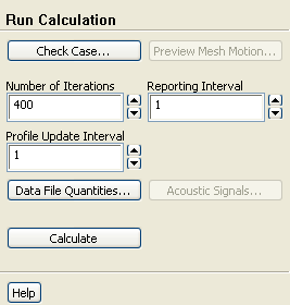
5.   Start the calculation by requesting 400 iterations.

Run Calculation

(a)   Enter 400 for Number of Iterations.

(b)   Click Calculate.

   During the calculation, ANSYS FLUENT will report that there is reversed flow occurring at the exit. This is due to the sudden expansion, which results in a recirculating flow near the exit.

The solution will converge in approximately 170 iterations (when all residuals have dropped below 0.001).

6.   Save the case and data files ( blower2.cas.gz and blower2.dat.gz).

File $\rightarrow$ Write $\rightarrow$ Case & Data...

Note:    It is good practice to save the case file whenever you are saving the data. This will ensure that the relevant parameters corresponding to the current solution data are saved accordingly.