Step 10: Postprocessing

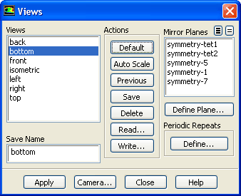
1.   Reset the view to the default view if you changed the default display of the mesh.

Graphics and Animations Views...

(a)   Click Default in the Actions group box and close the Views dialog box.

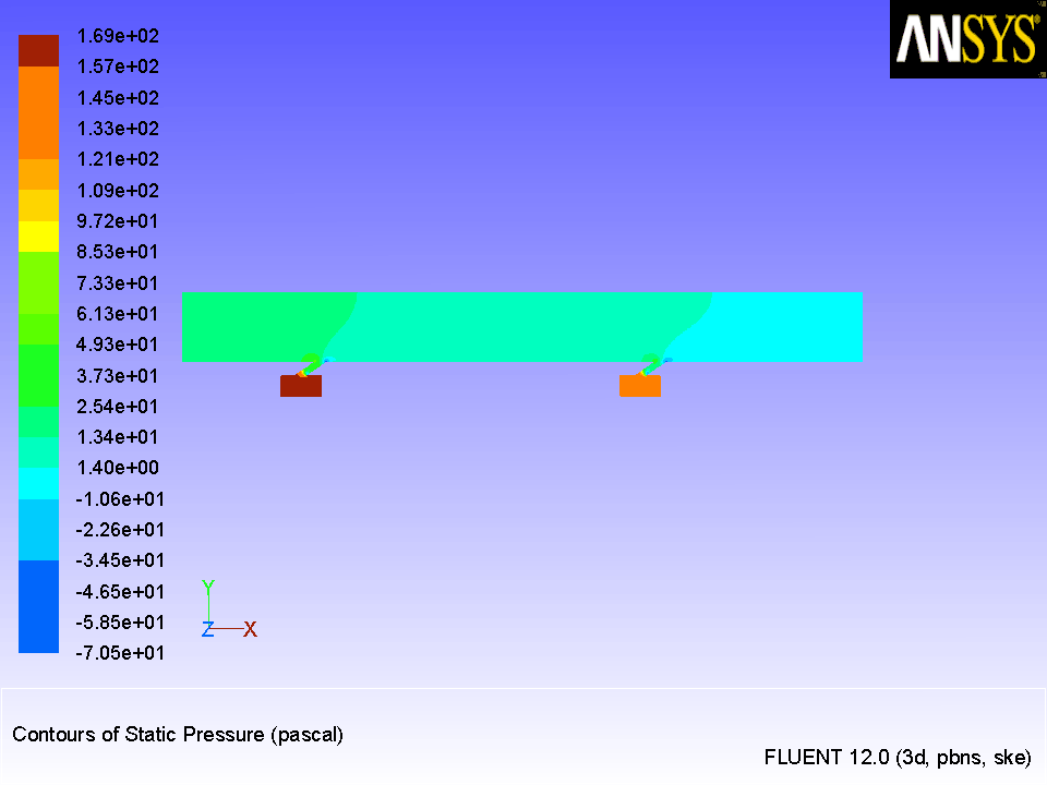
2.   Display filled contours of static pressure (Figure  7.5).

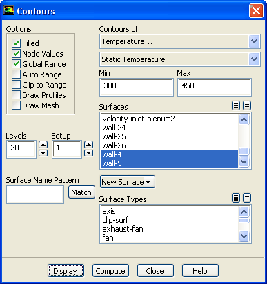
Graphics and Animations Contours Set Up...

(a)   Enable Filled in the Options group box.

(b)   Make sure Pressure... and Static Pressure are selected from the Contours of drop-down lists.

(c)   Select interface-duct, interface-hole1, interface-hole2, symmetry-1, symmetry-tet1, symmetry-tet2, wall-4, and wall-5 in the Surfaces selection list.

  Use the scroll bar to access the surfaces that are not initially visible in the Contours dialog box.

(d)   Click Display in the Contours dialog box.

Figure 7.5: Contours of Static Pressure

  The maximum pressure change (see Figure  7.5) is only 239 Pa. Compared to a mean pressure of 1.013e5 Pa, the variation is less than 0.3%, and thus the use of the incompressible ideal gas law is appropriate.

(e)   Zoom in on the view to display the contours at the holes (Figures  7.6 and 7.7).

Figure 7.6: Contours of Static Pressure at the First Hole

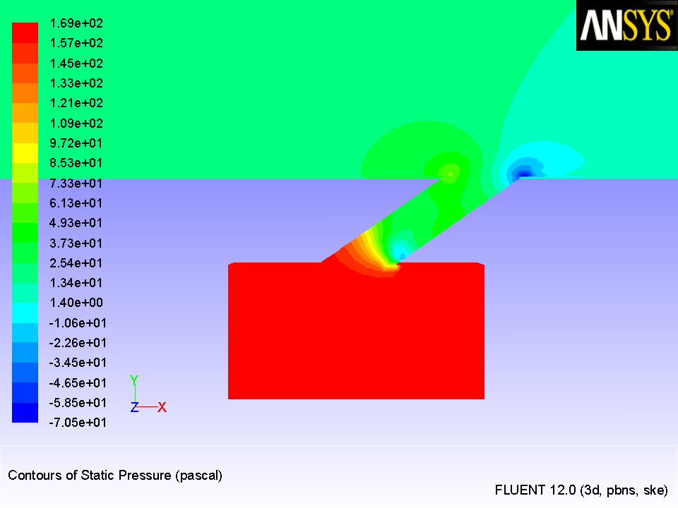Figure 7.7: Contours of Static Pressure at the Second Hole

  Note the high/low pressure zones on the upstream/downstream sides of the coolant hole, where the jet first penetrates the primary flow in the duct.

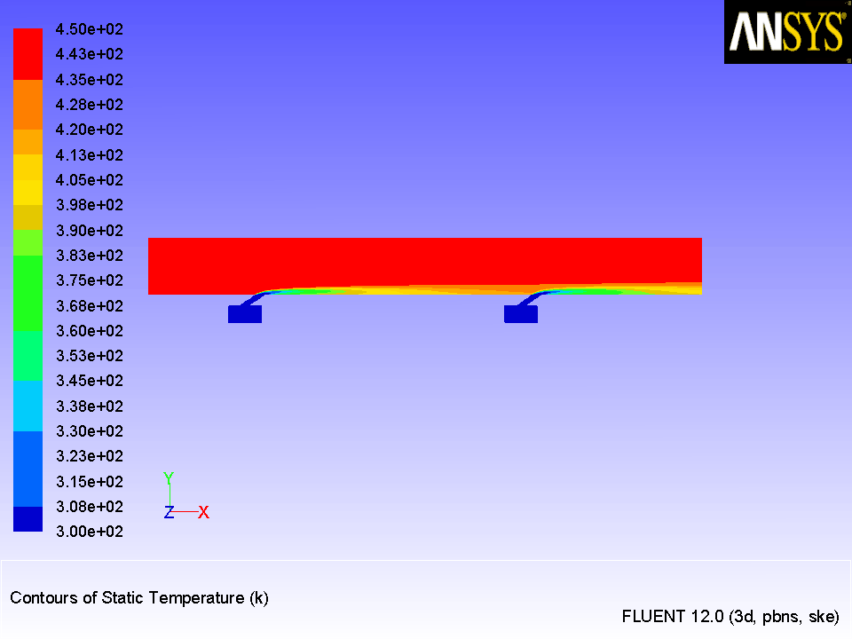
3.   Display filled contours of static temperature (Figures  7.8 and 7.9).

Graphics and Animations Contours Set Up...

(a)   Select Temperature... and Static Temperature from the Contours of drop-down lists.

(b)   Disable Auto Range in the Options group box so that you can change the maximum and minimum temperature gradient values to be plotted.

(c)   Enter 300 for Min and 450 for Max.

(d)   Disable Clip to Range in the Options group box.

(e)   Make sure that, interface-duct, interface-hole1, interface-hole2, symmetry-1, symmetry-tet1, symmetry-tet2, wall-4, and wall-5, are selected from the Surfaces selection list.

(f)   Click Display and close the Contours dialog box.

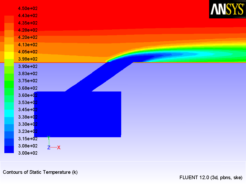
Figure 7.8: Contours of Static Temperature

(g)   Zoom in on the view to get the display shown in Figure  7.9.

Figure 7.9: Contours of Static Temperature (Zoomed-In View)

  Figures  7.8 and 7.9 clearly show how the coolant flow insulates the bottom of the duct from the higher-temperature primary flow.

4.   Display the velocity vectors (Figure  7.10).

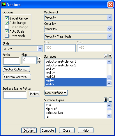
Graphics and Animations Vectors Set Up...

(a)   Make sure Velocity... and Velocity Magnitude are selected from the Color by drop-down lists.

(b)   Enable Auto Range in the Options group box

(c)   Enter 2 for the Scale.

  This enlarges the displayed vectors, making it easier to view the flow patterns.

(d)   Make sure that, interface-duct, interface-hole1, interface-hole2, symmetry-1, symmetry-tet1, symmetry-tet2, wall-4, and wall-5, are selected from the Surfaces selection list.

  Use the scroll bar to access the surfaces that are not initially visible in the dialog box.

(e)   Click Display and close the Vectors dialog box.

(f)   Zoom in on the view to get the display shown in Figure  7.10.

  In Figure  7.10, the flow pattern in the vicinity of the coolant hole shows the level of penetration of the coolant jet into the main flow. Note that the velocity field varies smoothly across the non-conformal interface.

Figure 7.10: Velocity Vectors

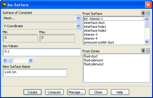
5.   Create an isosurface along a horizontal cross-section of the duct, 0.1 inches above the bottom, at $y$ = 0.1 in.

Surface $\rightarrow$ Iso-Surface...

(a)   Select Mesh... and Y-Coordinate from the Surface of Constant drop-down lists.

(b)   Enter 0.1 for Iso-Values.

(c)   Enter y=0.1in for New Surface Name.

(d)   Click Create.

(e)   Close the Iso-Surface dialog box.

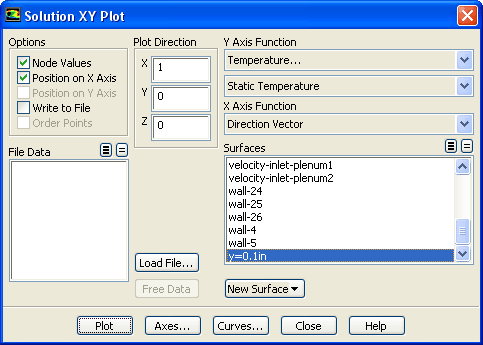
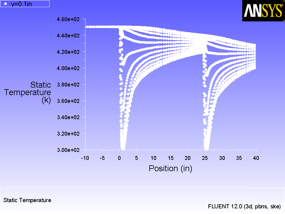
6.   Create an XY plot of static temperature on the isosurface created (Figure  7.11).

Plots XY Plot Set Up...

(a)   Retain the default values in the Plot Direction group box.

(b)   Select Temperature... and Static Temperature from the Y-Axis Function drop-down lists.

(c)   Select y=0.1in in the Surfaces selection list.

  Scroll down using the scroll bar to access y=0.1in.

(d)   Click Plot.

  In Figure  7.11, you can see how the temperature of the fluid changes as the cool air from the injection holes mixes with the primary flow. The temperature is coolest just downstream of the holes. You can also make a similar plot on the lower wall to examine the wall surface temperature.

(e)   Close the Solution XY Plot dialog box.

Figure 7.11: Static Temperature at $y$=0.1 in