Step 9: Solution

1.   Set the solution parameters.

Solution Methods

(a)   Select Second Order Upwind from the Momentum, Turbulent Kinetic Energy, Turbulent Dissipation Rate, and Energy drop-down lists in the Spatial Discretization group box.

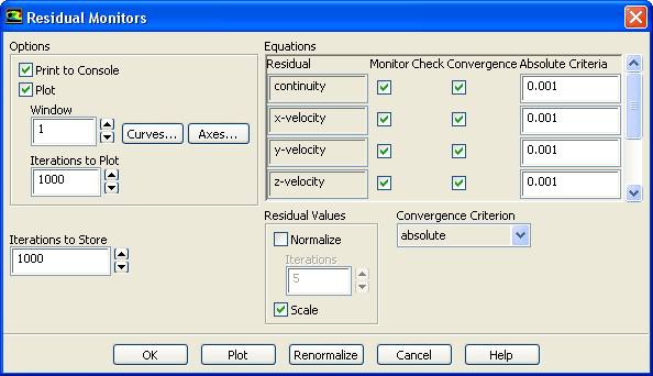
2.   Enable the plotting of residuals.

Monitors Residuals Edit...

(a)   Make sure Plot is enabled in the Options group box.

(b)   Click OK to close the Residual Monitors panel.

3.   Initialize the solution.

Solution Initialization

(a)   Select velocity-inlet-duct from the Compute from drop-down list.

(b)   Click Initialize.

4.   Save the case file ( filmcool.cas.gz).

File $\rightarrow$ Write $\rightarrow$ Case...

5.   Start the calculation by requesting 250 iterations.

Run Calculation

(a)   Enter 250 for the Number of Iterations.

(b)   Click Calculate.

Note:   During the first few iterations, the console reports that turbulent viscosity is limited in a couple of cells. The console should no longer display this message as the solution converges and the turbulent viscosity approaches more reasonable levels.

  The solution converges after approximately 125 iterations.

6.   Save the case and data files ( filmcool.cas.gz and filmcool.dat.gz).

File $\rightarrow$ Write $\rightarrow$ Case & Data...

Note:   If you choose a file name that already exists in the current folder, ANSYS FLUENT will prompt you for confirmation to overwrite the file.