Step 10: Iterate for Higher Divisions

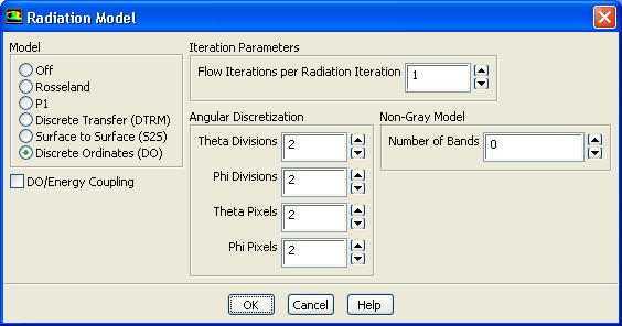
1.   Retain the default division as a base for comparison.

Models Radiation Edit...

(a)   Retain both Theta Divisions and Phi Divisions as 2.

(b)   Enter a value of 3 for Theta Pixels and Phi Pixels

(c)   Click OK to close the Radiation Model dialog box.

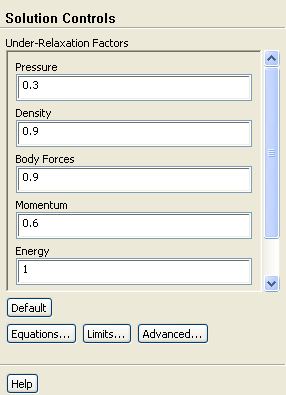
2.   Set the under-relaxation factors.

Solution Controls

(a)   Enter 0.9 for Density.

(b)   Enter 0.9 for Body Forces.

(c)   Enter 0.6 for Momentum.

3.   Request 1000 more iterations.

Run Calculation

  The solution will converge in approximately 80 iterations.

4.   Save the case and data files ( do_2x2_3x3_div.cas.gz and do_2x2_3x3_div.dat.gz).

File $\rightarrow$ Write $\rightarrow$ Case & Data...

5.   Display temperature profiles for the lens-inner.

Plots XY Plot Set Up...

(a)   Select all the files from the File Data selection list.

(b)   Click Free Data to remove the files from the list.

(c)   Retain the settings for Y axis Function and X axis Function.

(d)   Select lens-inner from the Surfaces selection list.

(e)   Click Plot.

(f)   Enable Write to File and click the Write... button to open the Select File dialog box.

i.   Enter do_2x2_3x3_div.xy for XY File and close the Select File dialog box.

6.   Repeat the procedure for 3 Theta Divisions and Phi Divisions.

(a)   Save the file as do_3x3_3x3_div.xy.

7.   Save the case and data files ( do_3x3_3x3_div.cas.gz and do_3x3_3x3_div.dat.gz).

File $\rightarrow$ Write $\rightarrow$ Case & Data...

8.   Repeat the procedure for 5 Theta Divisions and Phi Divisions.

(a)   Save the file as do_5x5_3x3_div.xy.

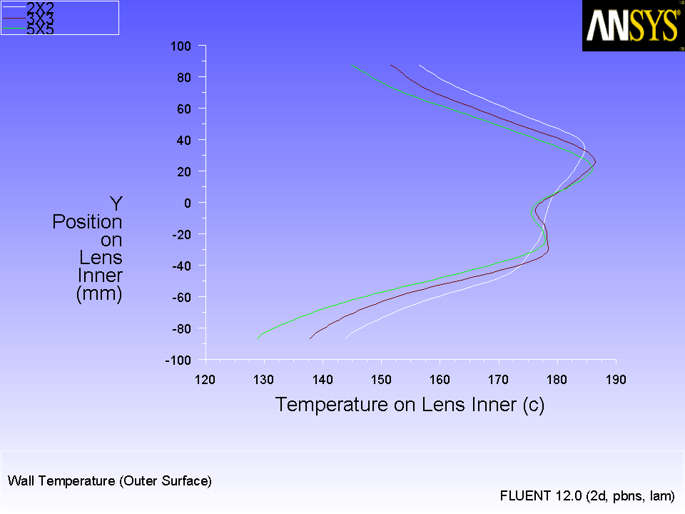
9.   Read in all the files for Theta Divisions and Phi Divisions of 2, 3, and 5 and display temperature profiles.

   Make sure you deselect lens-inner from the Surfaces list so that no plots are duplicated.

Figure 6.9: Temperature Profiles for Various Theta Divisions

10.   Save the case and data files ( do_5x5_3x3_div.cas.gz and do_5x5_3x3_div.dat.gz).

File $\rightarrow$ Write $\rightarrow$ Case & Data...

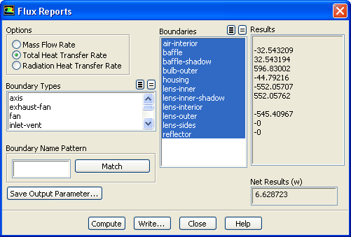
11.   Compute the total heat transfer rate.

Reports Fluxes Set Up...

(a)   Select Total Heat Transfer Rate in the Options group box.

(b)   Select all zones from the Boundaries selection list.

(c)   Click Compute.

Note:   The net heat load is 6.629 W, which equates to an imbalance of approximately 1.1% when compared against the heat load of the bulb.

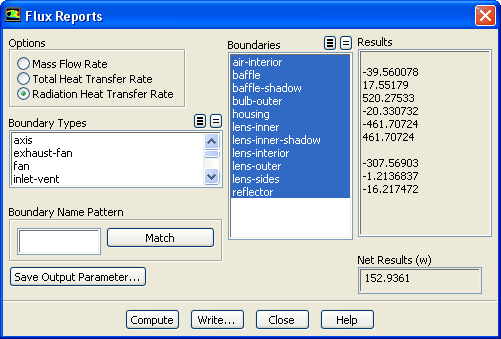
12.   Compute the radiation heat transfer rate.

Reports Fluxes Set Up...

(a)   Select Radiation Heat Transfer Rate in the Options group box.

(b)   Retain the selection of all boundary zones from the Boundaries selection list.

(c)   Click Compute and close the Flux Reports dialog box.

Note:   The net heat load is 152.9361.

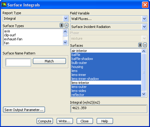
13.   Compute the radiation heat transfer rate incident on the surfaces.

Reports Surface Integrals Set Up...

(a)   Select Integral from the Report Type drop-down list.

(b)   Select Wall Fluxes... and Surface Incident Radiation from the Field Variable drop-down lists.

(c)   Select all surfaces except air-interior and lens-interior from the Surfaces selection list.

(d)   Click Compute.

  The incident load on lens-inner is slightly less than that on the reflector. This is because some radiation has been absorbed by the housing. However the incident load on the lens-outer is notably lower due to the amount of radiation which has been absorbed in the solid lens.

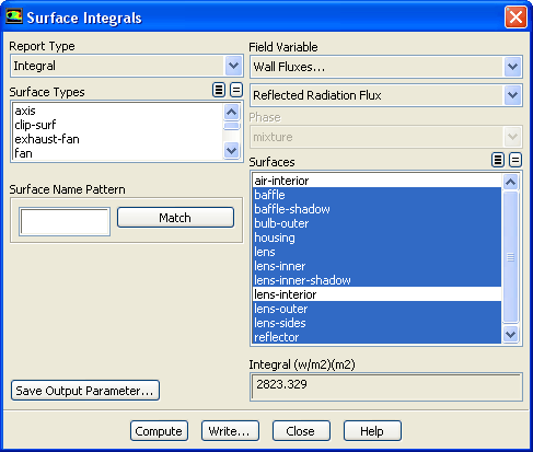
14.   Compute the reflected radiation flux.

Reports Surface Integrals Set Up...

(a)   Retain the selection of Integral from the Report Type drop-down list.

(b)   Select Wall Fluxes... and Reflected Radiation Flux from the Field Variable drop-down lists.

(c)   Select all surfaces except air-interior and lens-interior from the Surfaces selection list.

(d)   Click Compute.

  Reflected radiation flux values are printed in the console for all the zones. The zone baffle is facing the filament and its shadow ( baffle-shadow) is facing the lens. There is much more reflection on the filament side than on the lens side, as expected.

lens-inner is facing the fluid and lens-inner-shadow is facing the lens. Due to different refractive indexes and non-zero absorption coefficient on the lens, there is some reflection at the interface. Reflection on lens-inner-shadow is the reflected energy of the incident radiation from the lens side. Reflection on lens-inner is the reflected energy of the incident radiation from the fluid side.

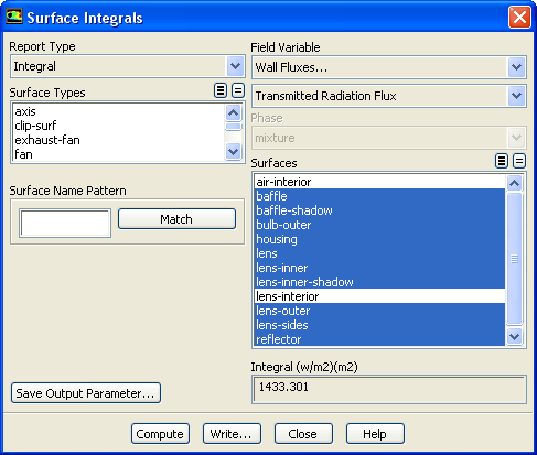
15.   Compute the transmitted radiation flux.

Reports Surface Integrals Set Up...

(a)   Retain the selection of Integral from the Report Type drop-down list.

(b)   Select Wall Fluxes... and Transmitted Radiation Flux from the Field Variable drop-down lists.

(c)   Ensure that all surfaces are selected except air-interior and lens-interior from the Surfaces selection list.

(d)   Click Compute.

  Transmitted radiation flux values are printed in the console for all the zones. All surfaces are opaque except lens. Zero transmission for all surfaces indicate that they are opaque.

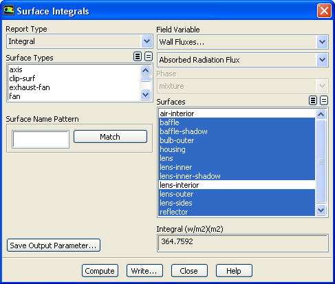
16.   Compute the absorbed radiation flux.

Reports Surface Integrals Set Up...

(a)   Retain the selection of Integral from the Report Type drop-down list.

(b)   Select Wall Fluxes... and Absorbed Radiation Flux from the Field Variable drop-down lists.

(c)   Ensure that all surfaces are selected except air-interior and lens-interior from the Surfaces selection list.

(d)   Click Compute.

(e)   Close the Surface Integrals dialog box.

   Absorption will only occur on opaque surface with a non-zero internal emissivity adjacent to participating cell zones. Note that absorption will not occur on a semi-transparent wall (irrespective of the setting for internal emissivity). In semi-transparent media, absorption and emission will only occur as a volumetric effect in the participating media with non-zero absorption coefficients.