Step 11: Adapting the Mesh

  The elbow solution can be improved further by refining the mesh to better resolve the flow details. In the following steps, you will adapt the mesh based on the temperature gradients in the current solution. Once the mesh is refined, you can continue the calculation.

1.   Adapt the mesh in the regions of high temperature gradient.

Adapt $\rightarrow$ Gradient...

(a)   Make sure that Refine is enabled in the Options group box.

   ANSYS FLUENT will not coarsen beyond the original mesh for a 3D mesh. Hence, it is not necessary to deselect Coarsen in this instance.

(b)   Select Temperature... and Static Temperature from the Gradients of drop-down lists.

(c)   Click Compute.

   ANSYS FLUENT will update the Min and Max values to show the minimum and maximum temperature gradient.

(d)   Enter 0.004 for Refine Threshold.

  It is a good rule of thumb to use 10 ${\rm\%}$ of the maximum gradient when setting the value for Refine Threshold.

(e)   Click Mark.

   ANSYS FLUENT will report in the console that approximately 940 cells were marked for adaption.

(f)   Click Manage... to open the Manage Adaption Registers dialog box.

i.   Click Display.

   ANSYS FLUENT will display the cells marked for adaption in the graphics window (Figure  1.15).

Figure 1.15: Cells Marked for Adaption

Extra:   You can change the way ANSYS FLUENT displays cells marked for adaption (Figure  1.16) by performing the following steps:

a.   Click Options... in the Manage Adaption Registers dialog box to open the Adaption Display Options dialog box.

b.   Enable Draw Mesh in the Options group box.

  The Mesh Display dialog box will open.

c.   Ensure that only the Edges option is enabled in the Options group box.

d.   Select Feature from the Edge Type list.

e.   Select all of the items except default-interior from the Surfaces selection list.

f.   Click Display and close the Mesh Display dialog box.

g.   Enable Filled in the Options group box in the Adaption Display Options dialog box.

h.   Enable Wireframe in the Refine group box.

i.   Click OK to close the Adaption Display Options dialog box.

j.   Click Display in the Manage Adaption Registers dialog box.

k.   Rotate the view and zoom in to get the display shown in Figure  1.16.

Figure 1.16: Alternative Display of Cells Marked for Adaption

l.   After viewing the marked cells, rotate the view back and zoom out again to return to the angle and magnification shown in Figure  1.13.

ii.   Click Adapt in the Manage Adaption Registers dialog box.

  A Question dialog box will open, confirming your intention to adapt the mesh. Click Yes to proceed.

Note:   There are two different ways to adapt. You can click Adapt in the Manage Adaption Registers dialog box as was just done, or close this dialog box and perform the adaption using the Gradient Adaption dialog box. If you use the Adapt button in the Gradient Adaption dialog box, ANSYS FLUENT will recreate an adaption register. Therefore, when the Manage Adaption Registers dialog box is open, use the Adapt button in it to save time.

iii.   Close the Manage Adaption Registers dialog box.

(g)   Close the Gradient Adaption dialog box.

2.   Display the adapted mesh (Figure  1.17).

General Display...

(a)   Make sure that All is selected from the Edge Type list.

(b)   Deselect all of the highlighted items from the Surfaces selection list except for symmetry.

(c)   Click Display and close the Mesh Display dialog box.

Figure 1.17: The Adapted Mesh

3.   (optional) Check the case to confirm that there are no recommendations for revisions to the setup.

Run Calculation Check Case

4.   Request an additional 150 iterations.

Run Calculation

  The solution will converge after approximately 100 additional iterations (Figures  1.18 and 1.19).

Figure 1.18: The Complete Residual History

Figure 1.19: Convergence History of Mass-Weighted Average Temperature

5.   Save the case and data files for the second-order solution with an adapted mesh ( elbow3.cas.gz and elbow3.dat.gz).

File $\rightarrow$ Write $\rightarrow$ Case & Data...

(a)   Enter elbow3.gz for Case/Data File.

(b)   Click OK to save the files and close the Select File dialog box.

  The files elbow3.cas.gz and elbow3.dat.gz will be saved in your default folder.

6.   Examine the filled temperature distribution (using node values) on the revised mesh (Figure  1.20).

Graphics and Animations Contours Set Up...

Figure 1.20: Filled Contours of Temperature Using the Adapted Mesh

7.   Display and save an XY plot of the temperature profile across the centerline of the outlet for the adapted second-order solution (Figure  1.21).

Plots XY Plot Set Up...

(a)   Disable Write to File in the Options group box.

  The button that was originally labeled Write... will change to Plot.

(b)   Make sure that Temperature... and Static Temperature are selected from the Y Axis Function drop-down lists.

(c)   Make sure that z=0_outlet is selected from the Surfaces selection list.

(d)   Click Plot.

Figure 1.21: Outlet Temperature Profile for the Adapted Second-Order Solution

(e)   Enable Write to File in the Options group box.

  The button that was originally labeled Plot will change to Write....

(f)   Click Write... to open the Select File dialog box.

i.   Enter outlet_temp3.xy for XY File.

ii.   Click OK to save the temperature data.

(g)   Close the Solution XY Plot dialog box.

8.   Display the outlet temperature profiles for each of the three solutions on a single plot (Figure  1.22).

Plots File Set Up...

(a)   Click the Add... button to open the Select File dialog box.

i.   Click once on outlet_temp1.xy, outlet_temp2.xy, and outlet_temp3.xy.

  Each of these files will be listed with their folder in the XY File(s) list to indicate that they have been selected.

Hint:   If you select a file by mistake, simply click the file in the XY File(s) list and then click Remove.

ii.   Click OK to save the files and close the Select File dialog box.

(b)   Select the folder path ending in outlet_temp1.xy from the Files selection list.

(c)   Enter 1st Order Soln in the lowest text-entry box on the right (next to the Change Legend Entry button).

(d)   Click the Change Legend Entry button.

  The item in the Legend Entries list for outlet_temp1.xy will be changed to 1st Order Soln. This legend entry will be displayed in the upper-left corner of the XY plot generated in a later step.

(e)   In a similar manner, change the legend entry for the folder path ending in outlet_temp2.xy to be 2nd Order Soln.

(f)   In a similar manner, change the legend entry for the folder path ending in outlet_temp3.xy to be Adapted Mesh.

(g)   Click Plot and close the File XY Plot dialog box.

  Figure  1.22 shows the three temperature profiles at the centerline of the outlet. It is apparent by comparing both the shape of the profiles and the predicted outer wall temperature that the solution is highly dependent on the mesh and solution options. Specifically, further mesh adaption should be used in order to obtain a solution that is independent of the mesh.

Figure 1.22: Outlet Temperature Profiles for the Three Solutions

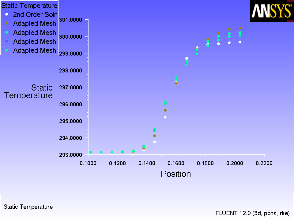
Extra:   You can perform additional rounds of mesh adaption based on temperature gradient and run the calculation to see how the temperature profile changes at the outlet. A case and data file ( elbow4.cas.gz and elbow4.dat.gz) has been provided in the solution_files folder, in which the mesh has undergone three more levels of adaption. The resulting temperature profiles have been plotted with outlet_temp2.xy and outlet_temp3.xy in Figure  1.23.

Figure 1.23: Outlet Temperature Profiles for Subsequent Mesh Adaption Steps

It is evident from Figure  1.23 that as the mesh is adapted further, the profiles converge on a mesh-independent profile. The resulting wall temperature at the outlet is predicted to be around 300.2  ${\rm K}$ after mesh independence is achieved. If the adaption steps had not been performed, the wall temperature would have incorrectly been estimated at around 299.75  ${\rm K}$.

If computational resources allow, it is always recommended to perform successive rounds of adaption until the solution is independent of the mesh (within an acceptable tolerance). Typically, profiles of important variables are examined (in this case, temperature) and compared to determine mesh independence.