Step 10: Postprocessing for the RNG $k$- $\epsilon$ Solution

1.   Plot the radial velocity distribution for the RNG $k$- $\epsilon$ solution and compare it with the distribution for the standard $k$- $\epsilon$ solution.

Plots XY Plot Set Up...

(a)   Enter 1 and 0 for X and Y respectively in the Plot Direction group box.

(b)   Select Velocity... and Radial Velocity from the Y Axis Function drop-down lists.

(c)   Select y=37cm and deselect wall-6 from the Surfaces selection list.

(d)   Disable the Write to File option.

(e)   Click the Load File... button to load the $k$- $\epsilon$ data.

i.   Select the file ke-data.xy in the Select File dialog box.

ii.   Click OK.

(f)   Click the Axes... button to open the Axes - Solution XY Plot dialog box.

i.   Enable Auto Range in the Options group box.

ii.   Click Apply and close the Axes - Solution XY Plot dialog box.

(g)   Click the Curves... button to open the Curves - Solution XY Plot dialog box, where you will define a different curve symbol for the RNG $k$- $\epsilon$ data.

i.   Retain 0 for the Curve #.

ii.   Select x from the Symbol drop-down list.

iii.   Click Apply and close the Curves - Solution XY Plot dialog box.

(h)   Click Plot in the Solution XY Plot dialog box (Figure  9.8).

Figure 9.8: Radial Velocity Distribution--RNG $k$- $\epsilon$ and Standard $k$- $\epsilon$ Solutions

  The peak velocity predicted by the RNG $k$- $\epsilon$ solution is higher than that predicted by the $k$- $\epsilon$ solution.This is due to the less diffusive character of the RNG $k$- $\epsilon$ model. Adjust the range of the $x$ axis to magnify the region of the peaks.

(i)   Click the Axes... button to open the Axes - Solution XY Plot dialog box, where you will specify the $x$-axis range.

i.   Disable Auto Range in the Options group box.

ii.   Retain the value of 0 for Minimum and enter 1 for Maximum in the Range dialog box.

iii.   Click Apply and close the Axes - Solution XY Plot dialog box.

(j)   Click Plot.

  The difference between the peak values calculated by the two models is now more apparent.

Figure 9.9: RNG $k$- $\epsilon$ and Standard $k$- $\epsilon$ Solutions ( $x=0$ cm to $x=1$ cm)

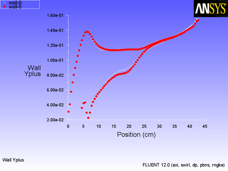
2.   Plot the wall y+ distribution on the rotating disk wall along the radial direction Figure  9.10.

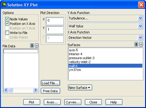
Plots XY Plot Set Up...

(a)   Select Turbulence... and Wall Yplus from the Y Axis Function drop-down lists.

(b)   Deselect y=37cm and select wall-6 from the Surfaces selection list.

(c)   Enter 0 and 1 for X and Y respectively in the Plot Direction group box.

(d)   Select any existing files that appear in the File Data selection list and click the Free Data button to remove the file.

(e)   Click the Load File... button to load the RNG $k$- $\epsilon$ data.

i.   Select the file ke-yplus.xy in the Select File dialog box.

ii.   Click OK.

(f)   Click the Axes... button to open the Axes - Solution XY Plot dialog box.

i.   Retain the default selection of X from the Axis group box.

ii.   Retain the default value of 0 for Minimum and enter 43 for Maximum in the Range group box.

iii.   Click Apply and close the Axes - Solution XY Plot dialog box.

(g)   Click Plot in the Solution XY Plot dialog box.

Figure 9.10: wall-6--RNG $k$- $\epsilon$ and Standard $k$- $\epsilon$ Solutions ( $x=0$ cm to $x=43$ cm)