Step 11: Compare a Contour Plot to the Display of a Variable on a Boundary

A contour plot with color bands has discrete colored regions while the display of a variable on a locator (such as a boundary) shows a finer range of color detail by default. The instructions that follow will illustrate a variable at the outlet and create a contour plot that displays the same variable at that same location.

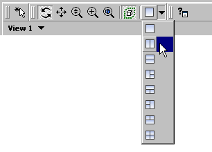
1.   To do the comparison, split the 3D Viewer into two viewports by using the Viewport Layout toolbar in the 3D Viewer toolbar:

2.   Right-click in both viewports and select Predefined Camera / View Towards -Y.

3.   In the Outline tree view, double-click on pressure outlet 7 (which is under elbow1 / fluid). The Details view of pressure outlet 7 appears.

4.   Click in the View 1 viewport.

5.   In the Details view for pressure outlet 7 on the Color tab:

(a)   Change Mode to Variable.

(b)   Ensure Variable is set to Pressure.

(c)   Ensure Range is set to Local.

(d)   Click Apply. The plot of pressure appears and the legend shows a smooth spectrum that goes from blue to red. Notice that this happens in both viewports; this is because Synchronize visibility in displayed views icon is enabled.

(e)   Click the Synchronize visibility in displayed views icon to disable this feature.

Now, add a contour plot at the same location:

1.   Click in View 2 to make it active, the title bar for that viewport becomes highlighted.

2.   In the Outline tree view, clear the check box beside fluid / pressure outlet 7.

3.   From the menu bar, select Insert/Contour.

4.   Accept the default contour name and click OK.

5.   In the Details view for the contour, ensure that the Locations setting is pressure outlet 7 and the Variable setting is Pressure.

6.   Set Range to Local.

7.   Click Apply. The contour plot for pressure appears and the legend shows a spectrum that steps through 10 levels from blue to red.

8.   Compare the two representations of pressure at the outlet. Pressure at the Outlet is on the left and a Contour Plot of pressure at the Outlet is on the right:

Figure 1.10: Boundary Pressure vs. a Contour Plot of Pressure

9.   Enhance the contrast on the contour bands:

(a)   In the Outline tree view, right-click on User Locations and Plots / Contour 2 and select Edit.

(b)   In the Details view for the contour, click on the Render tab, expand the Show Contour Lines area, and select the Constant Coloring check box. Then set the Color Mode to User Specified. Click Apply.

(c)   Click on the Labels tab and select Show Numbers. Click Apply.

10.   Explore the viewer synchronization options:

(a)   In View 1, click the cyan (ISO) sphere in the triad so that the two viewports show the elbow in different orientations.

(b)   In the 3D Viewer toolbar, click the Synchronize camera in displayed views icon . Both viewports take the camera orientation of the active viewport.

(c)   Clear the Synchronize camera in displayed views icon and click on the Z arrow head of the triad in View 1. The object again moves independently in the two viewports.

(d)   In the 3D Viewer toolbar, click the Synchronize visibility in displayed views icon .

(e)   In the Outline tree view, right-click on fluid / wall and select Show. The wall becomes visible in both viewports. (Synchronization applies only to events that take place after you enable the synchronize visibility function.)

11.   When you are done, use the viewport controller to return to a single viewport. The synchronization icons disappear.