In this example we shall investigate how to make a 3D simulation with OpenFOAM. The case we want to study is a steady turbulent flow circulating inside a room. This example introduces almost all the basic steps which should be done for studying a CFD problem and explains how these things can be carried out in a quite simple way in OpenFOAM.
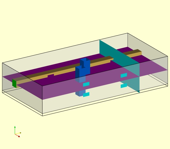
We want to study the motion of air circulating inside a room. The outline of the geometry is shown in Fig. 1. The room is crossed by a conduct. The air enters perpendicularly to one of the extremities of the conduct (inlet) at a velocity U = 0.5 m/s and flows out the other (outlet). There are two holes in the conduct and four small windows on one of the room walls through which the air can also flow. Two pillars are placed between the conduct and the wall with the windows.
|
|
As the case is steady-state and the fluid is supposed viscous and incompressible, the governing equations to be solved are:
|
We choosed the standard k - ε turbulence model with coefficients Cμ = 0.09, C1 = 1.44, C2 = 1.92, α k = 1, α ε = 7.69. In this model the velocity of the turbulent flow is estimated as a fluctuation around an average value: U = ‹ U › + U'; k = (1/2) |U'|2 represents the turbulent kinetic energy per unit of mass and ε the energy dissipation rate. We assume the fluctuations at the inlet to be isotropic and 5% of U, thus Ux = Uy = Uz = 0.5 ⋅ 0.05 = 25 ⋅ 10-3 m/s and k = 9.375 ⋅ 10-4 m2/s2. The energy dissipation is related to the turbulence scale l which we estimated to be 10% of 0.5 m, which is the width of the inlet. The value of ε is thus set to ε = (C μ 0.75 ⋅ k 3/2 )/l = 9.53 ⋅ 10 -5 m2/s3.
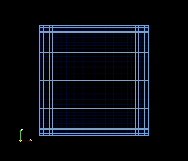
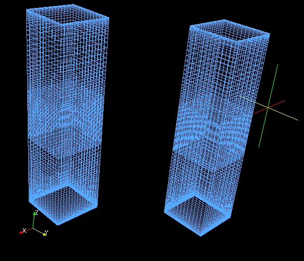
The mesh was generated by converting a .msh GAMBIT file according to the procedure described in the section Mesh conversion. The domain consists of about 5000000 cells. In Fig. 2 are shown some of the meshed patches of the domain.
|
|
|
|
|
|
The case requires initial and boundary conditions settings for all the involved fields: velocity U, pressure P, turbulent kinetic energy k and energy dissipation rate ε. The initial values for the fields are specified in the casename/0/fieldname files. The reader may consult the boundary conditions documentation section (in Italian) for more details. We report the rilevant sections of the fieldname files.
|
The initial velocity U has been set equal to 0.5 m/s in the y direction at the inlet:
|
We used the simpleFoam solver, implemented for steady incompressible flow. The numerical schemes for terms such as derivatives, interpolation procedures etc. are set in the casename/system/fvSchemes file. In this file we specify that the case is steady-state by giving the SteadyState value to the keyword timeScheme. The terms ∇ and ∇ 2 controlled respectively by the keywords gradSchemes and laplacianSchemes have been set to the value Gauss because we adopted the standard finite volume discretization of Gaussian integration which requires the interpolation of values from cell centres to face centres. The divergence term ∇ ⋅, controlled by the keyword divSchemes has been set to UD to ensure boundedness.
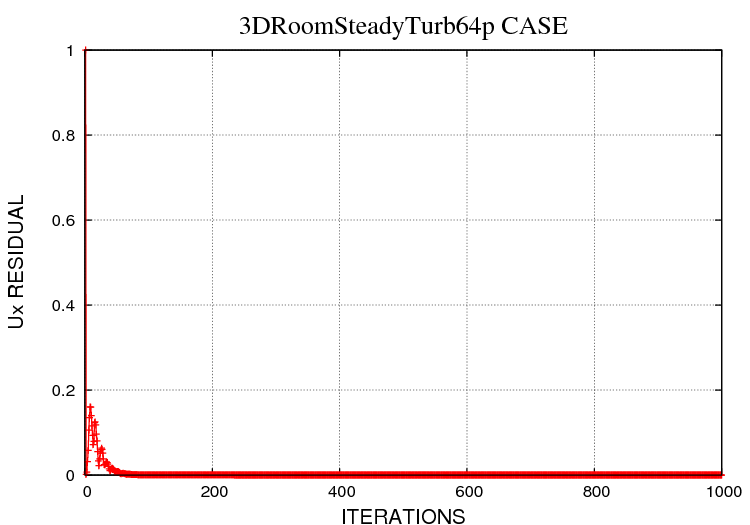
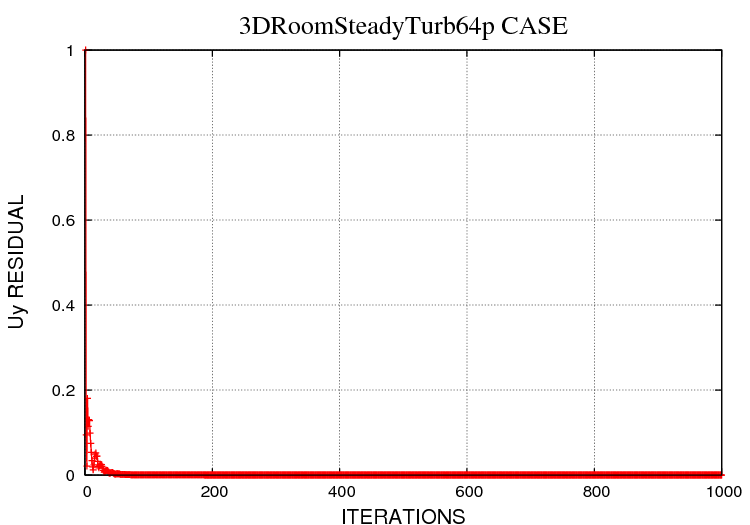
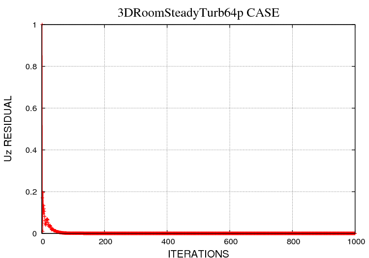
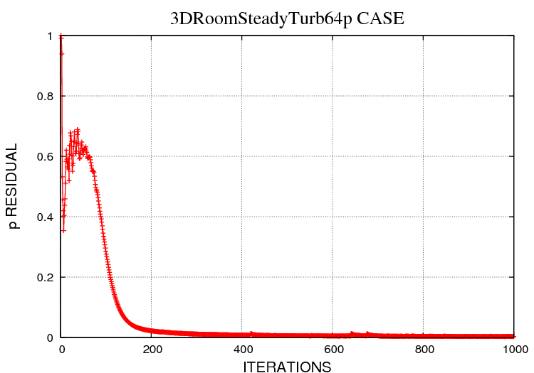
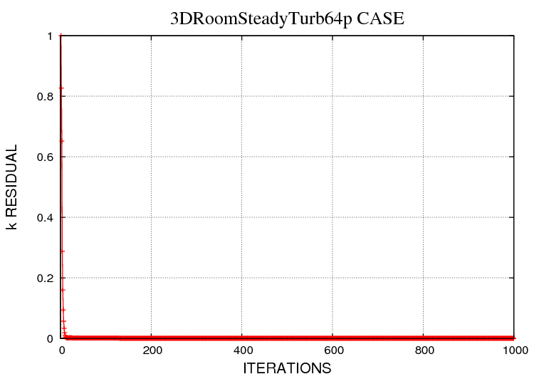
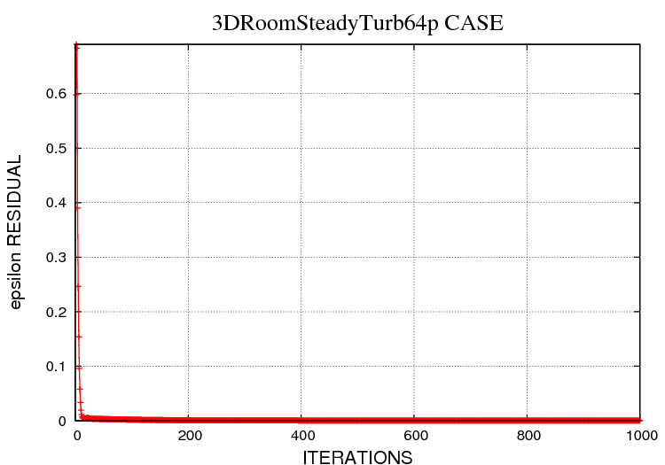
In Fig. 3 are shown the residuals of the involved fields after 1000 iterations. The case has been run in parallel using 64 cores.
|
|
|
|
|
|
|
|
Even if the maximum pressure gradient is only 0.5%, it is sufficient to cause a back flow with the air entering the room from the outlet as shown in Fig. 4.
|
|
|
The same simulation has been run with Fluent. In order to make a comparison we shall analyse the shape of the fields on two cutting planes, as shown in Fig. 5.
|
|
|
|
|
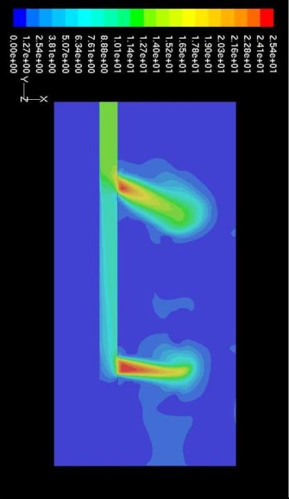
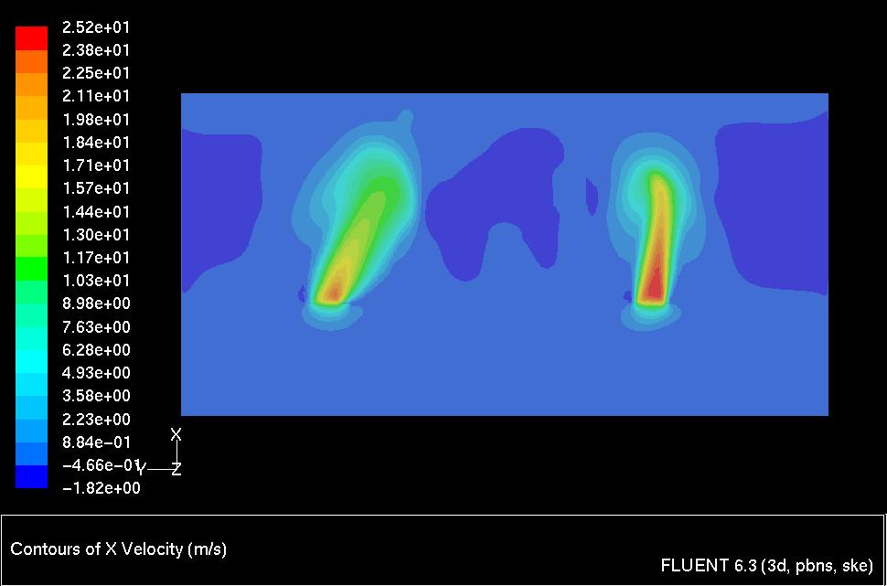
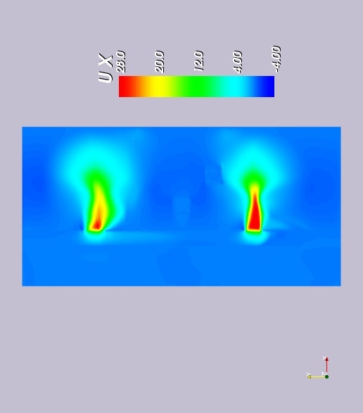
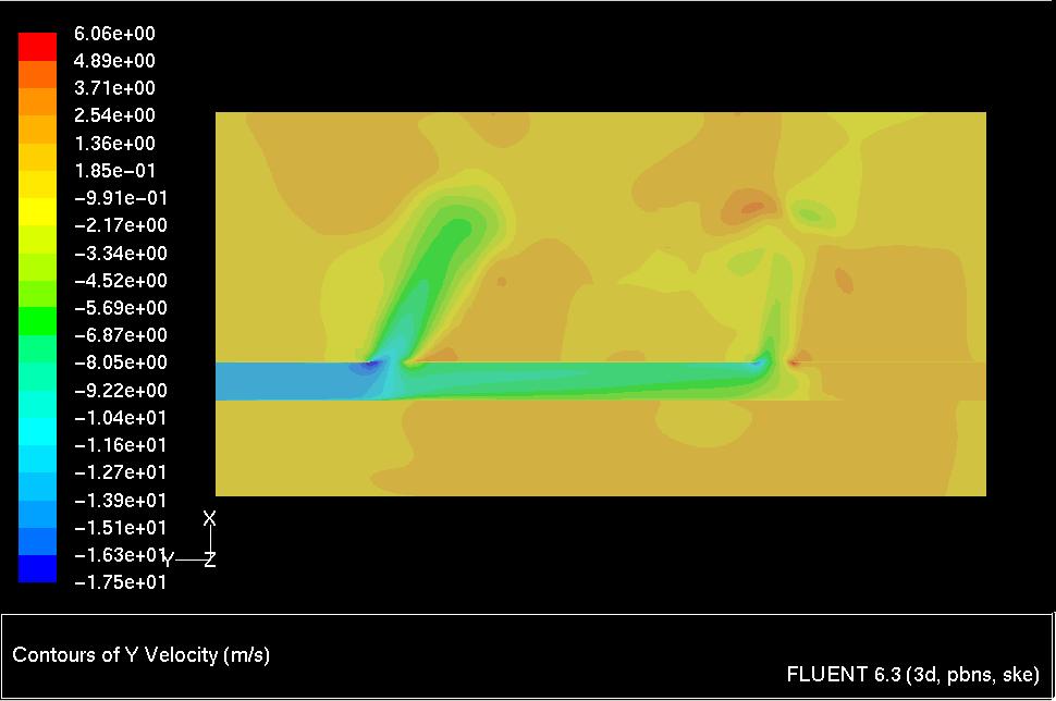
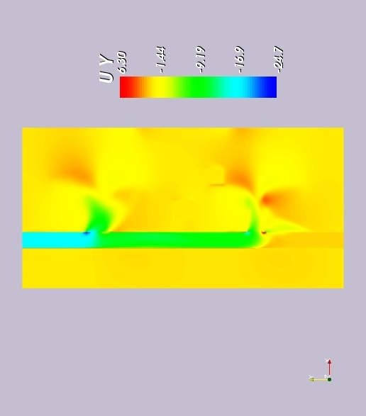
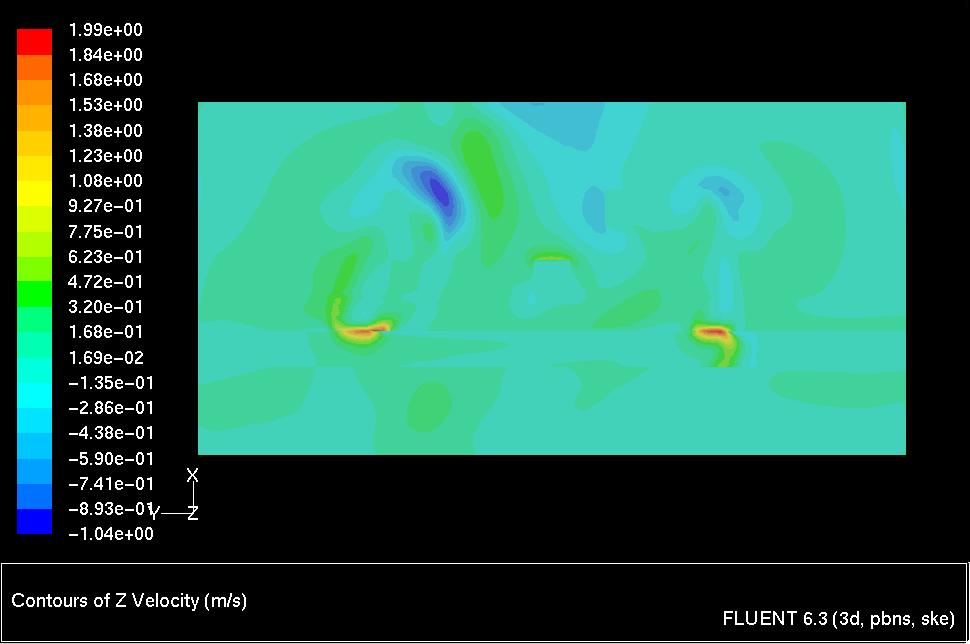
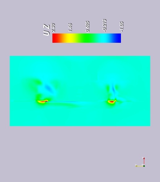
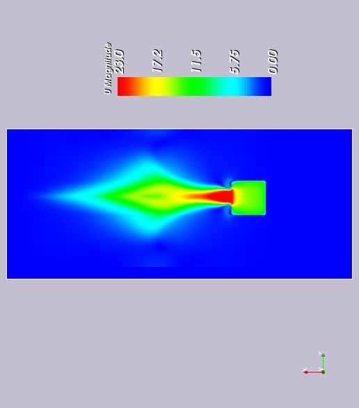
We observe that the magnitude of the velocity fields is of the same order. In the regions far from the two small holes placed on the conduct the velocity magnitude approaches to zero in both the two simulations. In the regions next to the conduct holes the velocity contour has a more diffusive shape in the OpenFOAM case. In Fig. 7 are shown the contour plots for the velocity components. An overall agreement is observed.
|
|
|
|
|
|
|
|
|
|
|
|
In Fig. 8 are shown the contour plots for the magnitude velocity field on the vertical plane. On average, the strength of the velocity fields at the conduct section are comparable. There is a nice agreement even for the size of the region where the velocity field doest not dump to zero.
|
|
|
|
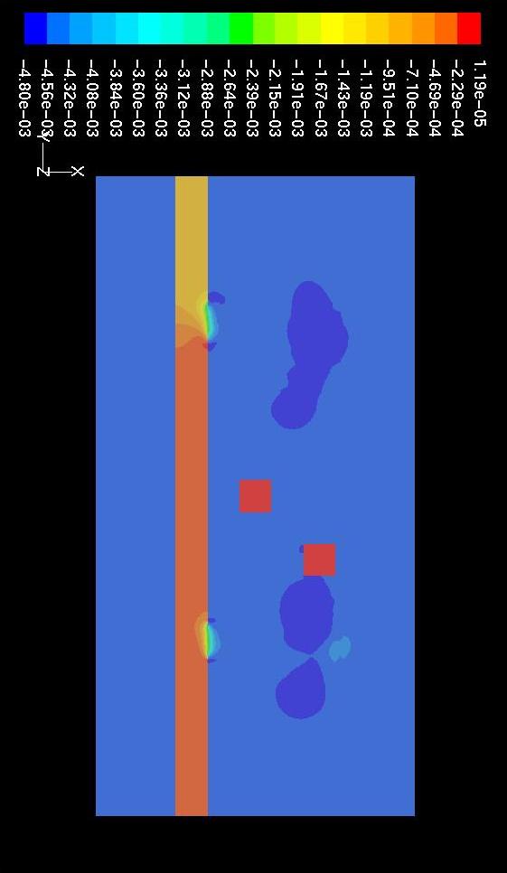
In Fig. 8 are shown the pressure contour plots on the horizontal plane. The Fluent picture reports (in Pa) the pressure gradient with respect to 1 atm = 101325 Pa as reference value, thus the negative values mean a value of pressure lower tham 1 atm. On the other hand the OpenFOAM picture reports (in Pa) the absolute pressure values as shown in the dispayed range. Hence in this case too there is an overall agreement.
|
|
|